Thoughts from the Swiss Photonics Machine Learning Workshop

Today I attended a machine learning workshop hosted by Swiss Photonics. The workshop was a small, day-long series of talks by industry experts in Neuchâtel, Switzerland, not far from Lausanne. I went to the workshop because a) I don't know much about machine learning and want to know more, and b) I wanted to connect with people within the Swiss Photonics circle. Most of the talks concerned deep learning for solving problems in industrial machine vision applications, such as quality control for the watch-making industry.

Here are the main things I learned, which may or not be correct. I welcome any opinions or corrections in the comments:

  • The term "learning" is used to mean "teaching a computer to recognize and classify patterns in data", such as finding people in images.
  • Learning involves finding patterns in data. Once patterns are idenfitied, a set of them can be combined to form a model. A model makes predictions about what future data may look like. This means that a model may be used to see whether new data meets our expectations. An example would be using pictures of products from a production line and searching for defects, i.e. those products that don't fit our classification of "good" products.
  • Learning applications require lots of training data to implement. This is where the primary cost of applying learning algorithms comes from.
  • There are three categories of learning: supervised, reinforced, and unsupervised.
  • The value in neural networks is their ability to make decisions in a way that is similar to humans. Other classification and decision algorithms work using strict programmatic rules and look for user-specified features. Neural networks do not require domain knowledge to establish features for a classifier. Their generality is their strength.
  • Deep learning just refers to really big neural networks. Neural networks are not new; recent hardware advances like GPU-based computation and the availability of large datasets are what has enabled Deep learning.

I did not hear much discussion about the tradeoffs and downsides to using neural networks or deep learning, other than that they require large amounts of training data. Notable talks were given by Reto Wyss of ViDi and Virginie Moser of http://www.csem.ch/site/. Wyss very eloquently explained why deep learning is useful for classification. Moser presented an extremely small and light-weight embedded machine vision system for traffic light control.
Approximating diffraction patterns of rectangular apertures with the FFT

A very common problem encountered by people learning Fourier optics or diffraction theory is the determination of the far field diffraction pattern from a rectangular aperture. This problem has a clean, analytical solution. Those who are familiar with MATLAB or a similar language may try to write computer code that calculates this diffraction pattern based on fast Fourier transform (FFT) implementations. Unfortunately, the output of the is code not, strictly speaking, the same as predicted by the analytical solution for a few reasons:

  1. The analytical solution is a function of continuous variables in space, whereas the simulated solution requires taking discrete samples of the relevant fields.
  2. The analytical solution is not band-limited. Therefore, aliasing will distort the computed solution.

In my last post I showed how to do basic pupil function simulations but did not go into many details about the FFT and possible errors associated with it. In this post I will dig a bit deeper into the topic of the FFT and its use in computational wave optics.

The purpose of this post is to investigate differences between the analytical theory and the simulated solution of the diffraction pattern from a rectangular aperture by investigating the simpler problem of diffraction from a 1D slit.

In [1]:
%pylab
%matplotlib inline
plt.style.use('dark_background')
plt.rcParams['image.cmap'] = 'plasma' 

from scipy.fftpack import fft
from scipy.fftpack import fftshift, ifftshift
Using matplotlib backend: Qt4Agg
Populating the interactive namespace from numpy and matplotlib

Scalar diffraction theory for a 1D slit

Goodman and many others have shown that the far-field (also known as Fraunhofer) solution to the diffracted electric field from a rectangular aperture is proportional to the Fourier transform of the field distribution in the aperture. This fact follows directly from applying the Fraunhofer approximation to the diffraction integral developed by Huygens and Fresnel (Goodman).

For both convenience and numerical efficiency, I will focus on the one-dimensional analog to this problem: diffraction from an infinitely-long slit with width $ a $. If there is an incident monochromatic plane wave with amplitude $E_0$ traveling in the z-direction perpendicular to a slit in the $z=0$ plane, then the Fraunhofer diffraction pattern for the field is expressed by the equation

$$U \left(x', z \right) = \frac{e^{jkz} e^{ jk\frac{x'^2}{2z} }}{\sqrt{j \lambda z}} \int_{-\infty}^{\infty} u \left( x, z = 0 \right) \exp \left( -j \frac{2 \pi}{\lambda z} xx'\right) dx $$

with $u \left( x, z = 0 \right) = E_0 $ denoting the incident field, $ k = \frac{2 \pi}{\lambda} $ representing the freespace wavenumber, $ x = 0 $ and $ x' = 0 $ the center planes of the slit and diffraction patterns, respectively, and $ j $ the imaginary number. The factor $ \sqrt{j \lambda z} $ comes from separating the solution to the 2D Huygens-Fresnel integral into two, 1D solutions. The irradiance in the z-planes after the slit is proportional to the absolute square of the field,

$$I \left( x', z \right) \propto \left| U \left( x', z \right) \right|^2$$

Taking the absolute square eliminates the complex exponentials preceding the integral so that the irradiance profile becomes

$$I \left( x', z \right) \propto \frac{1}{\lambda z} \left| \int_{-\infty}^{\infty} u \left( x \right) \exp \left( -j \frac{2 \pi}{\lambda z} xx'\right) dx \right|^2 = \frac{1}{\lambda z} \left| \mathcal{F} \left[ u \left( x, z \right) \right] \left( \frac{x'}{\lambda z}\right) \right|^2 $$

This expression means that the irradiance describing the Fraunhofer diffraction pattern from slit is proportional to the absolute square of the Fourier transform of the field at the aperture evaluted at spatial frequencies $ f_{x} = x' / \lambda z$. To arrive at the analytical solution, we perform the integration over a region where the slit is not opaque, $ \left[ -a/2, a/2 \right] $. Inside this region, the field is simply $ u \left( x \right) = E_0 $ because we have a monochromatic plane wave with this amplitude.

$$ \mathcal{F}\left[ u \left( x, z \right) \right] = \int_{-a/2}^{a/2} E_0 \exp \left( -j \frac{2 \pi}{\lambda z} xx'\right) dx $$

The analytical solution to this integral is

$$ \mathcal{F}\left[ u \left( x, z \right) \right] = a E_0 \text{sinc} \left( \frac{ax'}{\lambda z} \right) $$

where $ \text{sinc} \left( x \right) = \frac{\sin{\pi x}}{\pi x}$. The far-field irradiance is therefore the absolute square of this quantity divided by the product of the wavelength and the propagation distance.

Let's plot the analytically-determined irradiance profile of the diffraction pattern:

In [2]:
# Create a sinc function to operate on numpy arrays
def sinc(x):
    if (x != 0):
        # Prevent divide-by-zero
        return np.sin(np.pi * x) / (np. pi * x)
    else:
        return 1
sinc = np.vectorize(sinc)

amplitude    = 1     # Volt / sqrt(micron)
slitWidth    = 5     # microns
wavelength   = 0.532 # microns
propDistance = 10000 # microns (= 10 mm)

x = np.arange(-10000, 10000, 1)
F = sinc(slitWidth * x / wavelength / propDistance)
I = amplitude / (wavelength * propDistance) * (slitWidth * F)**2

plt.plot(x, I, linewidth = 2)
plt.xlim((-5000, 5000))
plt.xlabel(r'Position in observation plane, $\mu m$')
plt.ylabel('Power density, $V^2 / \mu m$')
plt.grid(True)
plt.show()

We can also verify a few key properties of the Fourier transform and ensure that our units are correct. The most important property is the conservation of energy, which in signal processing is often known as Parseval's theorem. In our case, conservation of energy means that the integral of the field over the slit must equal the integral of the field in any arbitrary z-plane.

$$\int_{-\infty}^{\infty} \left| u \left( x, z = 0 \right) \right|^2 dx = \int_{-\infty}^{\infty} \left| U \left( x', z \right) \right|^2 dx'$$

where the spatial frequency is $ f_{x} = \frac{x'}{\lambda z} $. Because the incident field is a plane wave, the integral over the slit is just the square of the plane wave amplitude multiplied by the slit width:

$$\int_{-a/2}^{a/2} E_0^2 dx = aE_0^2$$

We need the square integral to be proportional to units of power, which will be true if the field has units of $ \frac{\text{Volts}}{\sqrt{\mu m}} $ and not the more familiar $ \frac{\text{Volts}}{\mu m} $. This peculiarity stems from the fact that we're looking at a somewhat synthetic 1D case. With this in mind, the square integral has units of $ \text{Volts}^2 $ and is proportional to the power delivered by the plane wave.

The absolute square of the diffracted field is

$$ \left| U \left( x', z \right) \right|^2 = \frac{a^2 E_0^2}{\lambda z} \text{sinc}^2 \left( \frac{a x'}{\lambda z} \right)$$

The integral of $ \text{sinc}^2 \left( x \right) $ with my definition of $ \text{sinc} \left( x \right) $ over the real number line is just 1, so

$$ \int_{-\infty}^{\infty} \left| U \left( x', z \right) \right|^2 dx' = \frac{a^2 E_0^2}{\lambda z} \times \frac{\lambda z}{a} = aE_0^2$$

All of this is essentially a verification that our units and prefactors have most likely been handled correctly. Most Fourier optics texts drop a lot of prefactors in their derivations, so it's always good to check that they've done everything correctly :)

In [3]:
from scipy.integrate import simps
# Compute input power
powerIn  = slitWidth * amplitude**2

# Compute output power by numerical integration of the sinc
prefactor    = slitWidth **2 * amplitude**2 / wavelength / propDistance
sincIntegral = simps(F, x)
powerOut     = prefactor * sincIntegral

print('The input power is {0:.4f} square Volts. The output power is {1:.4f} square Volts'.format(powerIn, powerOut))
The input power is 5.0000 square Volts. The output power is 5.0373 square Volts

Simulating slit diffraction with the FFT

Can we simply use the FFT in Python's Scipy or in MATLAB to arrive at the same solution as above, skipping the math in the process? Let's try it.

We'll start by defining a square slit centered at the origin with the same width as above. The incident field is a plane wave with amplitude $E_0 = 1 \, V / \sqrt{m} $.

In [4]:
x     = np.linspace(-50, 50, num = 1024)
field = np.zeros(x.size, dtype='complex128') # Ensure the field is complex

field[np.logical_and(x > -slitWidth / 2, x <= slitWidth / 2)] = amplitude + 0j

plt.plot(x, np.abs(field), '.')
plt.xlabel(r'x-position, $\mu m$')
plt.ylabel(r'Field amplitude, $V / \sqrt{\mu m}$')
plt.ylim((0, 1.5))
plt.grid(True)
plt.show()

Now, it's important to really understand that this slit is represented in computer memory as a discrete sequence of field samples, not a continous curve. If we zoom in on the slit, we can better appreciate this:

In [5]:
plt.plot(x, np.abs(field), '.')
plt.xlabel(r'x-position, $\mu m$')
plt.ylabel(r'Field amplitude, $V / \sqrt{\mu m}$')
plt.xlim((-3, 3))
plt.ylim((-0.5, 1.5))
plt.grid(True)
plt.show()

Let's go ahead now and compute the FFT of this sequence of field samples. We first need to figure out what the units of the FFT are going to be. The sampling frequency $f_S$ for this field is simply 1 divided by the distance between each sample. The FFT outputs an array of numbers from spatial frequency 0 up to $ \left( \frac{N-1}{N} \right) f_S $. By default, the length of the output array $ N $ is the same as the length of the input. In Python, array indexes start from 0, so the relationship between index $ i $ and spatial frequency is

$$ f_{x} = \frac{f_S}{N} i $$

(In MATLAB, array indexes start at 1 so $i$ above should be replaced by $i - 1$ .)

We also need to do two other things when computing the numerical Fourier transform. First, we need to shift the input field using the fftshift command for arrays with an even number of elements and ifftshift for arrays with an odd number of elements. This will shift the elements of the array so that the point corresponding to x = 0 lies in the first element of the array (index 0).

The second thing we must do is multiply the fft results by the grid spacing dx to ensure that the scaling on the y-axis is correct.

In [6]:
dx = x[1] - x[0] # Spatial sampling period, microns
fS = 1 / dx      # Spatial sampling frequency, units are inverse microns
f  = (fS / x.size) * np.arange(0, x.size, step = 1) # inverse microns

diffractedField = dx * fft(fftshift(field)) # The field must be rescaled by dx to get the correct units

# Plot the field up to the Nyquist frequency, fS / 2
plt.plot(f[f <= fS / 2], np.abs(diffractedField[f <= fS / 2]), '.', linewidth = 2)
plt.xlim((0, fS / 2))
plt.xlabel(r'Spatial frequency, $\mu m^{-1}$')
plt.ylabel(r'Field amplitude, $V / \sqrt{\mu m}$')
plt.grid(True)
plt.show()

OK, so far so good. Let's now put the results in a format that is more easily compared to the analytical theory for the diffracted irradiance. We'll shift the FFT results back so that the peak is in the center using fftshift. (We also need to use fftshift here for arrays with an odd number of elements; typically, the order for odd elements is ifftshift -> fft -> fftshift.) We'll also rescale the x-axis by multiplying by $ \lambda z $ to get $x'$ and plot the theoretical result on top.

In [7]:
xPrime   = np.hstack((f[-(f.size/2):] - fS, f[0:f.size/2])) * wavelength * propDistance

IrradTheory = amplitude / (wavelength * propDistance) * \
    (slitWidth * sinc(xPrime * slitWidth / wavelength / propDistance))**2
IrradFFT    = fftshift(diffractedField * np.conj(diffractedField)) / wavelength / propDistance

plt.plot(xPrime, np.abs(IrradFFT), '.', label = 'FFT')
plt.plot(xPrime, IrradTheory, label = 'Theory')
plt.xlim((-5000, 5000))
plt.xlabel(r'x-position, $\mu m$')
plt.ylabel(r'Power density, $V^2 / \mu m$')
plt.grid(True)
plt.legend()
plt.show()
/home/douglass/anaconda3/lib/python3.5/site-packages/ipykernel/__main__.py:1: DeprecationWarning: using a non-integer number instead of an integer will result in an error in the future
  if __name__ == '__main__':

Not too bad! It looks like the simulation and the FFT agree pretty well. But, if we zoom in to some regions of the curve, you can see some discrepancies:

In [8]:
fig, (ax0, ax1) = plt.subplots(nrows = 1, ncols = 2, sharey = False, figsize = ((8,6)))

ax0.plot(xPrime, np.abs(IrradFFT), '.', label = 'FFT')
ax0.plot(xPrime, IrradTheory, label = 'Theory', linewidth = 2)
ax0.set_xlim((-500, 500))
ax0.set_ylim((0.002, 0.005))
ax0.set_xlabel(r'x-position, $\mu m$')
ax0.set_ylabel(r'Power density, $V^2 / \mu m$')
ax0.grid(True)

ax1.plot(xPrime, np.abs(IrradFFT), '.', label = 'FFT')
ax1.plot(xPrime, IrradTheory, label = 'Theory', linewidth = 2)
ax1.set_xlim((-2250, -1750))
ax1.set_ylim((0.000, 0.0004))
ax1.set_xlabel(r'x-position, $\mu m$')
ax1.grid(True)
ax1.legend()

plt.tight_layout()
plt.show()

Considering the discrepancy between the results and the theory, the following question comes to mind:

Is the discrepancy between the theoretical and FFT results due to numerical rounding errors, how we defined the slit, or something else?

How well do the theory and FFT results agree?

Let's start to answer this question by plotting the percent error between the theory and the FFT results.

In [9]:
percentError = np.abs((IrradTheory - IrradFFT) / IrradTheory) * 100

plt.semilogy(xPrime, percentError)
plt.xlabel(r'x-position, $\mu m$')
plt.ylabel('Percent error')
plt.xlim((-20000, 20000))
plt.grid(True)
plt.show()

Now that's interesting. The percent error varies wildly and spans nearly six orders of magnitude! Furthermore, it appears like the error actually gets slightly worse near the edge of the range, as evidenced by the upwards trend in the positive peaks. Finally, the fact that the percent error appears to have some sort of periodicity suggests that the discrepancies are not due to round-off errors but rather something else.

Does aliasing cause the disagreement?

Let's first see whether aliasing is causing a problem. The slit is not bandlimited, which means that its Fourier spectrum is infinite in extent. For this reason, we can never sample the slit at high-enough frequencies to and calculate its spectrum without aliasing artifacts. We can however, see if fidelity improves by increasing the sampling rate.

In [10]:
# Increase samples to approximately 1 million (2^20)
xNew        = np.linspace(-50, 50, num = 2**20)
fieldNew    = np.zeros(xNew.size, dtype='complex128') # Ensure the field is complex

fieldNew[np.logical_and(xNew > -slitWidth / 2, xNew <= slitWidth / 2)] = amplitude + 0j

plt.plot(xNew, np.abs(fieldNew), '.')
plt.xlabel(r'x-position, $\mu m$')
plt.ylabel(r'Field amplitude, $V / \sqrt{\mu m}$')
plt.ylim((0, 1.5))
plt.grid(True)
plt.show()
In [11]:
dxNew = xNew[1] - xNew[0] # Spatial sampling period, microns
fS    = 1 / dxNew         # Spatial sampling frequency, units are inverse microns
f     = (fS / xNew.size) * np.arange(0, xNew.size, step = 1) # inverse microns
xPrimeNew   = np.hstack((f[-(f.size/2):] - fS, f[0:f.size/2])) * wavelength * propDistance

diffractedField = dxNew * fft(fftshift(fieldNew)) # The field must be rescaled by dx to get the correct units

IrradTheoryNew = amplitude / (wavelength * propDistance) * \
    (slitWidth * sinc(xPrimeNew * slitWidth / wavelength / propDistance))**2
IrradFFTNew    = fftshift(diffractedField * np.conj(diffractedField)) / wavelength / propDistance

plt.plot(xPrimeNew, np.abs(IrradFFTNew), '.', label = 'FFT')
plt.plot(xPrimeNew, IrradTheoryNew, label = 'Theory')
plt.xlim((-5000, 5000))
plt.xlabel(r'x-position, $\mu m$')
plt.ylabel(r'Power density, $V^2 / \mu m$')
plt.grid(True)
plt.legend()
plt.show()
/home/douglass/anaconda3/lib/python3.5/site-packages/ipykernel/__main__.py:4: DeprecationWarning: using a non-integer number instead of an integer will result in an error in the future

Now the agreement looks much better! Here's the new percent error with $ 2^{20} $ samples compared to the old one with $ 2^{10} $.

In [12]:
percentErrorNew = np.abs((IrradTheoryNew - IrradFFTNew) / IrradTheoryNew) * 100

plt.semilogy(xPrime,    percentError,       label = r'$N = 2^{10}$', linewidth = 2)
plt.semilogy(xPrimeNew, percentErrorNew, label = r'$N = 2^{20}$')
plt.xlabel(r'x-position, $\mu m$')
plt.ylabel('Percent error')
plt.xlim((-20000, 20000))
plt.grid(True)
plt.legend(loc = 'lower right')
plt.show()

Here we see that increasing the sampling rate by nearly three orders of magnitude (1024 samples vs. 1,048,576) improves the relative error at the origin and at the points where the error was already low to begin with. However, it does nothing to improve the error at the peaks in the plot, the first two peaks lying approximately 1000 microns on either side of the origin.

Just aliasing, or something more?

We can begin to better understand the differences between the computational solution and the analytical solution by first underlining these two facts:

  1. The diffracted far-field is a continous Fourier transform of the continuous field distribution in the aperture.
  2. The FFT produces a discrete Fourier transform (DFT) of the sampled field in the aperture.

Since the analytical solution and the FFT solution come from two related but different mathematical operations, should we have expected to get the right answer in the first place? As others have pointed out, the discrete time Fourier transform (DTFT) of a square function is a ratio of two sines, not a sinc. Furthermore, the DFT (and equivalently the FFT result) is simply a sampled version of the DTFT. Therefore, we might expect that sampling the DTFT solution for a square wave will produce the same results as the FFT solution. Let's go ahead and try it.

According to Wikipedia, and changing variables to agree with my notation above, the DTFT solution of the square wave is

$$F \left( f_{x} \right) = \frac{\sin \left[ \pi f_{x} \left( M + 1 \right) \right] }{\sin \left( \pi f_{x} \right) } e^{ -j \pi f_{x} M }, \, M \in \mathbb{Z} $$

where $ M $ is an integer and $ f\_{x} $ is the spatial frequency. An important property of the DTFT is that it is periodic between 0 and 1. If I had used the angular spatial frequency $ k\_{x} = 2 \pi f\_{x} $ the periodicity would be between 0 and $ 2 \pi $. With this information, we can map our spatial frequency vector onto the appropriate range for the DTFT.

The square function corresponding to this DTFT solution is defined with the left edge of the square starting at the origin:

$$ f \left( x \right) = \text{rect} \left( \frac{n - M/2}{M} \right) , \, M \in \mathbb{Z}, \, n = 0, 1, \ldots, N - 1$$

$ n $ is the index of the samples taken from the square and $ M $ denotes the center of the square. So, to use this expression for the DTFT of the square, we will first need to shift our original input so that the left edge of the square is at the origin.

In [13]:
numSamples = 2**20 # Large numbers of samples needed to make FFT and DTFT agree
x          = np.linspace(0, 100, num = numSamples)
field      = np.zeros(x.size, dtype='complex128') # Ensure the field is complex

field[x <= slitWidth] = amplitude + 0j
M                     = np.sum(np.real(field) / amplitude) # Only works if input field is real and ones.

plt.plot(x, np.abs(field), '.')
plt.xlabel(r'x-position, $\mu m$')
plt.ylabel(r'Field amplitude, $V / \sqrt{\mu m}$')
plt.ylim((0, 1.5))
plt.grid(True)
plt.show()

print('M is {0:.0f}.'.format(M))
M is 52429.
In [14]:
def rectDTFT(f, M):
    # Returns the DTFT of a rect centered at M
    if (f != 0):
        return np.sin(f * np.pi * (M + 1)) \
             / np.sin(f * np.pi)           \
             * np.exp(-1j * f * np.pi * M)
    else:
        return (M + (1 + 0j))
rectDTFT = np.vectorize(rectDTFT)

# Compute the diffracted field with the FFT
dx = x[1] - x[0]
fS = 1 / dx
f  = (fS / x.size) * np.arange(0, x.size, step = 1) # inverse microns
diffractedField = dx * fft(fftshift(field))

# Sample the DTFT of a rectangular slit
dx_DTFT  = x[1] - x[0]
fS_DTFT  = 1 / dx_DTFT
fDTFT    = np.linspace(0, 1, num = numSamples, endpoint = False) # For plotting the DTFT

plt.plot(f[f <= fS / 2],  np.abs(diffractedField[f <= fS / 2]), linewidth = 2, label = 'FFT')
plt.plot(fDTFT * fS_DTFT, dx_DTFT * np.abs(rectDTFT(fDTFT, M)), '.',           label = 'DTFT')
plt.xlim(0,5)
plt.ylim(0,6)
plt.xlabel(r'Spatial frequency, $\mu m^{-1}$')
plt.ylabel(r'Field amplitude, $V / \sqrt{ \mu m}$')
plt.grid(True)
plt.legend()
plt.show()

I placed the x- and y-axes to display a similar range as the equivalent plot above. We see that the DTFT result, which is the ratio of two sine waves, is also in good agreement with the FFT. So now we have the FFT and the DTFT of the field at the aperture modeling the diffraction pattern reasonably well.

How well does the DTFT match the analytical results? Let's look at their percent error and compare it to the one between the analytical theory and the FFT for $ 2^{20} $ samples.

In [15]:
IrradDTFT = dx_DTFT**2 * fftshift(rectDTFT(fDTFT, M) * np.conj(rectDTFT(fDTFT, M))) / wavelength / propDistance
    
percentErrorDTFT = np.abs(IrradTheoryNew - IrradDTFT) / IrradTheoryNew * 100

plt.semilogy(xPrimeNew, percentErrorNew,  label = r'FFT vs. Theory, $N = 2^{20}$', linewidth = 2)
plt.semilogy(xPrimeNew, percentErrorDTFT, label = r'DTFT vs. Theory, $N = 2^{20}$')
plt.xlabel(r'x-position, $\mu m$')
plt.ylabel('Percent error')
plt.xlim((-20000, 20000))
plt.grid(True)
plt.legend(loc = 'lower left')
plt.show()

What the above plot shows is that the error between the analytical theory and both the FFT and DTFT predictions are practically the same. This means that the FFT is computing the DTFT of the field at the aperture and not the continuous Fourier transform. The DTFT result is therefore inherently including the aliasing artifacts that prevent accurate computation of the diffracted field with the FFT.

Despite the large relative errors, we still get pretty good results with both the FFT and DTFT predictions around the origin so long as the sampling frequency is large, or, equivalently, the grid spacing is small:

In [16]:
plt.plot(xPrimeNew, IrradTheoryNew,   label = 'Theory', linewidth = 2)
plt.plot(xPrimeNew, IrradFFTNew, '.', label = 'FFT')
plt.plot(xPrimeNew, IrradDTFT,   '^', label = 'DTFT',   markersize = 8, alpha = 0.5)
plt.xlim((-5000, 5000))
plt.grid(True)
plt.legend()
plt.show()
/home/douglass/anaconda3/lib/python3.5/site-packages/numpy/core/numeric.py:474: ComplexWarning: Casting complex values to real discards the imaginary part
  return array(a, dtype, copy=False, order=order)

Summary

This entire exercise effectively showed that it is impossible to compute an exact diffraction pattern from a slit with a straight-forward approach based on the fast Fourier transform. There are two ways of looking at why this is, though they are both effectively based in the same underlying ideas.

  1. The spectrum of a slit is not band limited, so aliasing will always distort the FFT calculation.
  2. The FFT is computing the discrete time Fourier transform, not the continuous Fourier transform.

Because the slit is not band limited, frequencies in the spectrum that are larger than the field's sampling frequency are effectively folded back into and interfere with the spatial frequencies that are less than the sampling frequency. This creates differences between the analytical theory and its computed estimate.

Similarly, if we pay close attention to the analytical theory, we find that the diffraction pattern results from a continuous Fourier transform. The FFT however computes discrete samples of the discrete time Fourier transform. These are two similar, but fundamentally different things. Importantly, the DTFT result includes the aliasing artifacts by its very nature; it is a periodic summation of the continuous Fourier transform of the field, and this periodic summation results in overlapping tails of the spectra.

If anything, I hope this post clarifies a commmon misconception in Fourier optics, namely that we can compute exact diffraction patterns with the FFT algorithm.

Simulating microscope pupil functions

*Note: I remade this post to address minor inconsistencies and what I perceived to be a lack of attention to units of some of the physical quantities. The updated post may be found here.

Simple simulations of microscope pupil functions

In one of my recent publications, my co-authors and I investigated an aberration that is especially pernicious for 3D localization microscopies such as STORM and PALM. This aberration results in a dependence of the perceived position of a single, fluorescent molecule on its axial position within the focal plane of a microscope. To identify a possible source for this aberration, I employed a phase retrieval algorithm to obtain the pupil function of the microscope. I then decomposed the pupil function into a number of orthogonal polynomial terms and identified the specific terms that led to the aberration that we observed. In this case, terms associated with coma were the culprits.

So why exactly is coma bad for 3D localization microscopy? Unfortunately, we did not have time to go into the subtleties question in the publication due deadlines on the revisions. Luckily, the internet is a wonderful tool for explaining some of these ideas outside of the formal structure of an academic paper, which is what I will do here.

To answer the question, we first require a bit of knowledge about Fourier optics. The purpose of this post is to describe what a pupil function is and how it can be easily simulated on a computer with Python. We'll then see how we can use it to model a simple aberration: defocus. A future post will explain why coma is bad for 3D localization microscopy using the foundations built upon here.

Pupil Function Basics

The pupil function of a microscope (and really, of any optical system) is an important tool for analyzing the aberrations present in the system. The pupil function is defined as the two dimensional Fourier transform of the image of an isotropic point source. The two dimensional Fourier transform of a function of two variables x and y is expressed as

$$F \left( k_x, k_y \right) = \iint f \left( x, y \right) \exp \left[ -j \left( k_{x}x + k_{y}y \right) \right] dx dy$$

(I was originally trained as an engineer, so I tend to use 'j' for the imaginary number more than 'i'.) The inverse Fourier transform converts $F \left( k_x, k_y \right)$ back into $f \left( x, y \right)$ and is given by

$$f \left( x, y \right) = \iint F \left( k_x, k_y \right) \exp \left[ j \left( k_{x}x + k_{y}y \right) \right] dk_x dk_y$$

In this case, $x$ and $y$ are variables representing 2D coordinates in the image plane and $k_x$ and $k_y$ are the spatial frequencies. $f \left( x, y \right)$ and $F \left( k_x, k_y \right)$ are known as Fourier transform pairs.

An isotropic point source is an idealized source of electromagnetic radiation that emits an equal intensity in all directions. Strictly speaking, real sources such as atoms and molecules are dipoles and not isotropic emitters. This assumption is however a good model for collections of many fluorescent molecules possessing dipole moments that are all pointing in different directions and that are smaller than the wavelength of light because the molecules' individual emission patterns average out. It is also a good approximation for a dipole whose moment is randomly reorienting in many directions during an image acquisition due to thermally-induced rotational diffusion.

The image of a point source is known as the point spread function (PSF) of the microscope. In signal processing, it's known as a two dimensional impulse response.

The equation that relates the image of the isotropic point source to the pupil function $P \left( k_x, k_y \right)$ is

$$\text{PSF}_{\text{A}} \left( x, y \right) = \iint P \left( k_x, k_y \right) \exp \left[ -j \left( k_{x}x + k_{y}y \right) \right] dx dy$$

The subscript A on the PSF stands for amplitude and means that we are working with the electric field, not the irradiance. The irradiance, which is what a camera or your eye measures, is proportional to the absolute square of $\text{PSF}_{\text{A}}$. In words, the above equation restates the definition above: the pupil function and the amplitude PSF are Fourier transform pairs.

Simulating Diffraction Limited Pupil Functions and PSF's

We can simulate how an aberration affects the image of a point source by simulating an aberrated pupil function and computing the Fourier transform above to get the amplitude PSF. The easiest model to simulate is based on scalar diffraction theory, which means that we ignore the fact that the electromagnetic radiation is polarized (i.e. a vector) and treat it as a scalar quantity instead. Even though this is an approximation, it still can give us a good idea about the fundamental physics involved.

To perform the simulation, we must first discretize the continuous quantities in the Fourier transform. We'll model $\text{PSF}_{\text{A}}$ and $P \left( k_x, k_y \right)$ as discrete scalar quantities on 2D grids and perform a fast Fourier transform to turn the pupil function into the PSF.

In [1]:
# Load scientific Python libraries
%pylab
%matplotlib inline
from scipy.fftpack import fft2
from scipy.fftpack import fftshift, ifftshift
Using matplotlib backend: Qt4Agg
Populating the interactive namespace from numpy and matplotlib
In [2]:
plt.style.use('dark_background')
plt.rcParams['image.cmap'] = 'plasma' 

Let's start by setting up the image plane and spatial frequency grids. If we work with square images, then the primary quantity we have to set a value for is the number of pixels. The number of pixels that we choose to simulate is a bit arbitrary, though as we'll see later, it determines the spacing of the discretized pupil function coordinates.

In [3]:
imgSize = 513 # Choose an odd number to ensure rotational symmetry about the center

The rest of the important parameters for setting up the grids are determined by your microscope.

In [4]:
wavelength = 0.68 # microns
NA         = 1.4  # Numerical aperture of the objective
nImmersion = 1.51 # Refractive index of the immersion oil
pixelSize  = 0.1  # microns, typical for microscopes with 60X--100X magnifications

Now we have enough information to define the grid on which the pupil function lies.

In [5]:
kMax = 2 * pi / pixelSize # Value of k at the maximum extent of the pupil function
kNA  = 2 * pi * NA / wavelength
dk   = 2 * pi / (imgSize * pixelSize)

When working with discrete Fourier transforms, a common question that arises is "What are the units of the Fourier transform variable?" We can answer this question by these rules:

$k_{Max} \propto \frac{1}{dx}$

$x_{Max} \propto \frac{1}{dk}$

These two rules are just a manifestation of the Nyquist-Shannon sampling criterion: the maximum spatial frequency $ k\_{Max} $ is determined by the inverse of the sampling period in space $dx$, while the maximum size $x\_{Max}$ of the signal is proportional to the inverse of the period of spatial frequency samples $dk$. This is why the maximum spatial frequency above is $2 \pi / \text{pixelSize}$. I will go into more detail on this in a later post.

The pupil function of a microscope is non-zero for values of $\left( k_x, k_y \right)$ such that $k_x^2 + k_y^2 \leq \frac{2 \pi NA}{\lambda}$. The quantity $\frac{2 \pi NA}{\lambda}$ is represented by kNA above. The size of a pixel dk in spatial frequency units (radians per distance) is inversely proportional to the maximum size of the image in pixels, or imgSize * pixelSize. Likewise, the size of a pixel in microns is proportional to the inverse of the maximum size of the pupil function in spatial frequencies. This is just a manifestation of the properties of Fourier transform pairs.

In [6]:
kx = np.arange((-kMax + dk) / 2, (kMax + dk) / 2, dk)
ky = np.arange((-kMax + dk) / 2, (kMax + dk) / 2, dk)
KX, KY = np.meshgrid(kx, ky) # The coordinate system for the pupil function
print('kmin : {0}'.format(kx[0]))
print('kmax : {0}'.format(kx[-1]))
print('Size of kx : {0}'.format(kx.size))
kmin : -31.354686913020938
kmax : 31.354686913020036
Size of kx : 513

Now that the coordinate system for the pupil function is setup, we can go ahead and define the pupil function for an aberration free microscope. First, we need to create a mask whose value is one inside a circle whose extent is set by the microscope's NA and zero outside it. This mask is used to create a circular pupil.

In [7]:
maskRadius = kNA / dk # Radius of amplitude mask for defining the pupil
maskCenter = np.floor(imgSize / 2)
W, H       = np.meshgrid(np.arange(0, imgSize), np.arange(0, imgSize))
mask       = np.sqrt((W - maskCenter)**2 + (H- maskCenter)**2) < maskRadius

plt.imshow(mask, extent = (kx.min(), kx.max(), ky.min(), ky.max()))
plt.xlabel('kx, rad / micron')
plt.ylabel('ky, rad / micron')
plt.colorbar()
plt.show()

The pupil function is a complex quantity, which means it has both real and imaginary components. The unaberrated pupil function for an on-axis point source simply has a uniform phase and amplitude equal to one inside the mask.

In [8]:
amp   = np.ones((imgSize, imgSize)) * mask
phase = 2j * np.pi * np.ones((imgSize, imgSize))
pupil = amp * np.exp(phase)
In [9]:
fig, (ax0, ax1) = plt.subplots(nrows = 1, ncols = 2, sharey = True, figsize = (10,6))
img0 = ax0.imshow(amp, extent = ((kx.min(), kx.max(), ky.min(), ky.max())))
ax0.set_title('Pupil function amplitude')
ax0.set_xlabel('kx, rad / micron')
ax0.set_ylabel('ky, rad / micron')

img1 = ax1.imshow(np.imag(phase), extent = ((kx.min(), kx.max(), ky.min(), ky.max())))
ax1.set_title('Pupil function phase')
ax1.set_xlabel('kx, rad / micron')
plt.show()

The amplitude PSF for the isotropic point source is simply the Fourier transform of this pupil function. The camera, which measures irradiance and not electric field, sees the absolute square of the amplitude PSF.

In [10]:
psfA_Unaberrated = fftshift(fft2(ifftshift(pupil))) * dk**2
psf              = psfA_Unaberrated * np.conj(psfA_Unaberrated) # PSFA times its complex conjugate

zoomWidth = 5 # pixels

# It is important to set interpolation to 'nearest' to prevent smoothing
img = plt.imshow(np.real(psf), interpolation = 'nearest')
plt.xlim((np.floor(imgSize / 2) - zoomWidth, np.floor(imgSize / 2) + zoomWidth))
plt.ylim((np.floor(imgSize / 2) - zoomWidth, np.floor(imgSize / 2) + zoomWidth))
plt.xlabel('Position, pixels')
plt.ylabel('Position, pixels')
plt.colorbar(img)
plt.show()

This is a simulated image of an on-axis, in-focus, isotropic point source from an unaberrated pupil with an object-space pixel size of 100 nm.

The image is also a decent approximation of what a real single molecule image looks like in localization microscopies. I say decent because a single molecule will have a dipolar emission profile, not isotropic. Additionally, the scalar-diffraction model used here ignores polarization effects. Finally, a real image will have noise, which would be reflected as a random variation in the signal of each pixel.

Let's see how a line profile through the center of the image looks relative to the profile of the Airy disk, which is the mathematical solution to the diffraction pattern from a circular aperture in scalar diffraction theory. The Airy disk is given by

$$I \left( X \right) = I_{0} \left[ \frac{2J_{1} \left( X \right)}{X} \right]^2$$

where $J_{1} \left( X \right) $ is the Bessel function of the first kind and order 1 and $ X = \frac{2 \pi r (\text{NA})}{\lambda} $. Here, $r$ is the distance from the center of the image plane, so we can easily convert it to pixels.

Because the pupil of the microscope is circular and unaberrated, it is also the solution for PSF of the microscope.

In [11]:
from scipy.special import j1 as bessel1
px   = np.arange(-10, 11) # pixels
x    = 2 * np.pi * px * NA * pixelSize / wavelength 
airy = np.max(np.real(psf)) * (2 * bessel1(x) / x)**2

# Fix point at x = 0 where divide-by-zero occurred
airy[int(np.floor(x.size / 2))] = np.max(np.real(psf))

# Take a line profile through the center of the simulated PSF
lineProfile = np.real(psf[int(np.floor(imgSize / 2)), int(np.floor(imgSize / 2) - 10) : int(np.floor(imgSize / 2) + 11)])

plt.plot(px, airy,             linewidth = 4,  label = 'Airy disk')
plt.plot(px, lineProfile, 'o', markersize = 8, label = 'Simulated PSF')
plt.xlabel('Pixels')
plt.ylabel('Irradiance, a.u.')
plt.legend()
plt.show()
/home/douglass/anaconda3/lib/python3.5/site-packages/ipykernel/__main__.py:4: RuntimeWarning: invalid value encountered in true_divide

The simulated PSF agrees well with the scalar diffraction theory, demonstrating that we have correctly simulated the microscope's PSF from an unaberrated pupil function.

Defocus

Now that we can simulate the diffraction-limited image of an in-focus isotropic point source, let's add some defocus to demonstrate what the PSF would look like as the camera or sample is scanned along the axial direction.

Defocus can be added in numerous ways. One is to multiply our pupil function by the phase aberration for defocus, which is usually modeled as a parabolic phase aberration in the pupil coordinates. However, as I explained in a previous post, this is an approximate model for defocus and fails for large numerical apertures.

Another simple way is to propagate the plane wave angular spectrum in the image plane to nearby planes. This relatively easy method is used in a well-known microscopy paper (Hanser, 2004) and involves multiplying the pupil function by a defocus kernel before performing the Fourier transform.

$$\text{PSF}_{\text{A}} \left( x, y, z \right) = \iint P \left( k_x, k_y \right) \exp \left( j k_{z} z \right) \exp \left[ -j \left( k_{x}x + k_{y}y \right) \right] dx dy$$

Here, $k_z = \sqrt{\left( 2 \pi n / \lambda \right)^2 - k_x^2 - k_y^2}$. The defocus kernel essentially shifts the phase of each plane wave with pupil coordinates $\left( k_x, k_y \right)$ by an amount that depends on its coordinates and the distance from the image plane $z$.

The above equation means that we can model the PSF behavior as we scan through the focal plane by computing the defocus kernel for different distances from focus. Then, we multiply our perfect pupil by this defocus kernel and compute its Fourier transform to get the amplitude and irradiance PSF's.

In [12]:
# Defocus from -1 micron to + 1 micron
defocusDistance = np.arange(-1, 1.1, 0.1)
defocusPSF      = np.zeros((imgSize, imgSize, defocusDistance.size))

for ctr, z in enumerate(defocusDistance):
    # Add 0j to ensure that np.sqrt knows that its argument is complex
    defocusPhaseAngle   = 1j * z * np.sqrt((2 * np.pi * nImmersion / wavelength)**2 - KX**2 - KY**2 + 0j)
    defocusKernel       = np.exp(defocusPhaseAngle)
    defocusPupil        = pupil * defocusKernel
    defocusPSFA         = fftshift(fft2(ifftshift(defocusPupil))) * dk**2
    defocusPSF[:,:,ctr] = np.real(defocusPSFA * np.conj(defocusPSFA))

And that's it. All we needed to do was multiply pupil by the defocus kernel and compute the FFT like before. Now let's look at a couple of defocused PSF's at different distances from the focal plane.

In [13]:
fig, (ax0, ax1) = plt.subplots(nrows = 1, ncols = 2)

zoomWidth = 20 # pixels
indx      = [9, 14] # indexes to defocus distances to plot

# Find the maximum in the in-focus image for displaying PSF's on the correct intensity scale
maxIrradiance = np.max(defocusPSF[:,:,10])

ax0.imshow(defocusPSF[:, :, indx[0]], vmin =0, vmax = maxIrradiance, interpolation = 'nearest')
ax0.set_xlim((np.floor(imgSize / 2) - zoomWidth / 2, np.floor(imgSize / 2) + zoomWidth / 2))
ax0.set_ylim((np.floor(imgSize / 2) - zoomWidth / 2, np.floor(imgSize / 2) + zoomWidth / 2))
ax0.set_xlabel('x-position, pixels')
ax0.set_ylabel('y-position, pixels')
ax0.set_title('Defocus: {0:.2f} microns'.format(defocusDistance[indx[0]]))

ax1.imshow(defocusPSF[:, :, indx[1]], vmin =0, vmax = maxIrradiance, interpolation = 'nearest')
ax1.set_xlim((np.floor(imgSize / 2) - zoomWidth / 2, np.floor(imgSize / 2) + zoomWidth / 2))
ax1.set_ylim((np.floor(imgSize / 2) - zoomWidth / 2, np.floor(imgSize / 2) + zoomWidth / 2))
ax1.set_xlabel('x-position, pixels')
ax1.set_ylabel('y-osition, pixels')
ax1.set_title('Defocus: {0:.2f} microns'.format(defocusDistance[indx[1]]))
plt.tight_layout()
plt.show()

As more and more defocus is added to the pupil, the PSF gets dimmer because the same number of photons are spread out across a larger area of the detector.

In a future post I'll discuss how we can model arbitrary aberrations within this framework. The idea is similar to how defocus is implemented here: you find the phase profile for the aberration, multiply it by the unaberrated pupil, and finally compute the 2D Fourier transform.

Beware the paraxial approximation in microscopy

I have had a difficult time resolving what originally seemed to be an inconsistency between a 2004 research article about estimating microscope pupil functions and the body of knowledge concerning the theory of aberrations in optical systems.

In the article by Hanser, et al.[1], the authors utilize an imaging model for calculating the amplitude point-spread function of an optical system that incorporates defocus as an exponential term inside the Fourier transform integral:

\begin{equation*} \text{PSF}_{\text{A}} \left( x, y, z \right) = \iint_{pupil} P \left( k_x, k_y \right) e^{i k_z z} e^{i \left( k_{x}x + k_{y}y \right)} dk_x dk_y \end{equation*}

where \(k_z = \sqrt{\left( 2 \pi n / \lambda \right)^2 - \left( k_x^2 + k_y^2 \right)}\). (I changed the notation of some variables used in the text because the authors confusingly use \(k\) to represent spatial frequency in units of /cycles per distance/ instead of the much more common radians per distance.) In the image plane at \(z = 0\), there is no defocus and we get the amplitude point spread function (PSF) as the Fourier transform of the pupil function \(P \left( k_x, k_y \right)\) just like we would expect (see Goodman[2], Chapter 6, pp. 129-131).

The problem arises when I try to verify this model when \(z\) is not equal to zero by computing the defocused PSF using the wavefront error for defocus. From the scalar diffraction theory of aberrations, the defocused PSF is the Fourier transform of the pupil function multiplied by a phase factor whose phase angle is proportional to the wavefront error \(W \left( k_x, k_y \right)\)

\begin{equation*} \text{PSF}_{\text{A}} \left( x, y, z \right) = \iint_{pupil} P \left( k_x, k_y \right) e^{i k W \left( k_x, k_y \right)} e^{i \left( k_{x}x + k_{y}y \right)} dk_x dk_y \end{equation*}

Any textbook discussing Seidel aberrations will tell you that the defocused wavefront error \(W\) is quadratic in the pupil plane coordinates, i.e. \(W \sim k_x^2 + k_y^2\). Goodman even states this with little justification later in Chapter 6 on p. 149 when discussing defocus [2]. So how can I reconcile the first equation in which the defocus goes as the square root of a constant minus the squared pupil coordinates with the second equation that is quadratic in pupil coordinates?

The answer, as you might have guessed from the title of this post, is that /the Seidel polynomial term for defocus is a result of applying the paraxial approximation when computing the wavefront error/. You can see this by calculating the phase of a spherical wave in the pupil plane that is centered on the axis in the image plane; Goodman states it is quadratic without justification, but this is only true near the axis. Mahajan offers a geometrical interpretation of \(W\) on p. 148, where he notes that the path length difference for defocus "is approximately equal to the difference of sags of the reference sphere and the wavefront.[3]" He then goes on to derive the same expression for \(W\) that Goodman gets; he states the approximation that he uses, whereas Goodman implicitly assumes a quadratic phase front in the pupil. Hanser et al., on the other hand, are essentially propagating the plane wave angular spectrum from the image plane to nearby planes to model defocus. I think that this should be rigorously correct since no approximation is applied. For me, it is unfortunate that this was not made clear in their paper because I spent quite a bit of time trying to reconcile the two results.

The lesson of this story is to be sure you know about the approximations that go into a "standard" result found in textbooks. I falsely assumed that the Seidel aberrations were exact and that Hanser, et al. were suspect when in fact it was the other way around. Because the paraxial approximation is so widespread in optics theory, it can often lie hidden behind an equation and its effects can easily be taken for granted. This is a problem for the large NA systems used in microscopy where the results of the paraxial approximation are not often valid.

What's the difference between a back focal plane and pupil plane?

Yesterday in the lab I asked one of my colleagues whether she knew what the pupil plane of a microscope objective was. Her answer was no. I then unknowingly proceeded to give her a description which I now realize was false. I said that the pupil plane is the plane near the backside of the objective where the light intensity is proportional to the Fourier transform of the image. Later that evening, I realized that this explanation was, in fact, wrong. I had described to her what is the /back focal plane/ for an infinity-corrected objective.

Don't worry, I will correct myself when I see her later today. However, this experience does raise one important question that I have never seriously considered in optics: what is the meaningful difference between the pupil plane of an optical system and its back focal plane?

First, I should point out that there is no difference between a /back/ focal plane and one of the two focal planes of an objective; these are merely semantics that reflect the fact that we think of the sample as being in front of the objective. The back focal plane is therefore the focal plane of the objective located on the side opposite the sample. Now, everyone who has taken a Fourier optics class has probably learned the following mantra:

The focal plane of a lens contains the Fourier transform of the object.

Of course, this statement is usually what we remember, but in fact it should look more like this:

The focal plane of a lens contains the Fourier transform of the object, except for every other detail we ignore in the math.

While it's true that the light intensity here reflects the sample's two-dimensional Fourier transform, the general case often contains additional phase factors and expressions to account for the pupil size and apodization (see Goodman, section 5.2). Regardless, it is in the back focal plane where the light intensity cpontains information on the angular spectrum that makes up the object.

In contrast, the pupil plane contains either the image of the objective's aperture stop or the physical stop itself, depending on what sets the limit on the numerical aperture of the objective in the infinity space (again, see Goodman, appendix B). Moreover, the pupil plane is also used as the reference plane for quantifying the objective's aberrations. This is because, for a diffraction-limited system, the wavefront in the (exit) pupil plane will be a spherical wave converging towards the image of a point source and truncated by the aperture stop Goodman again discusses this in section 6.1). Deviations from the spherical reference wave serve as the means to quantify the aberrations in a system.

From an experimental point of view, the back focal plane is interesting because it is used in Fourier microscopy, for which many setups have been devised to image it (see Figure 1 in this excellent arXiv submission.) What I really am wondering now is how one would go about imaging the pupil plane as a means of exploring an objective's aberrations, and whether this is at all feasible.

Paraxial Optics (2): What problem does it solve?

Summary

  1. Paraxial optics is a tool to aid in building optical systems.
  2. Paraxial optics solves the imaging problem.
  3. The imaging problem concerns finding the location, size, and orientation of an image given an object and an optical system.
  4. An optical system is a collection of objects like lenses, mirrors, prisms, cameras, etc. that collects the light emitted or scattered by an object and delivers it to another location where it can be detected and processed for information.
  5. The rules of paraxial optics allow for a perfect imaging system, i.e. a system that creates a one-to-one correspondance between points in an object plane and an image plane.

Paraxial optics solves the imaging problem

In this post I will use paraxial optics to mean paraxial geometrical optics. This is important since the paraxial approximation can also apply to the wave theory of light.

When learning a new theory, I often find it most useful to first identify the problem that the theory was developed to solve. This approach is particularly pertinent for learning paraxial optics, since the theory is largely used as a tool to aid in the construction of optical systems. Unfortunately, the fact that paraxial optics can help solve problems often becomes lost on people because they never actually build anything for the purpose of imaging. And even if a someone never builds a camera or microscope, I think it is difficult for them to see what paraxial optics concepts--such as principle planes and aperture stops--can do for helping them troubleshoot their hardware when it is not working as expected.

So, with this in mind, I will use this part in a series of blog posts to answer the following question: what is the problem that paraxial optics solves?

Paraxial optics solves the imaging problem [1]. The imaging problem as I see it is simply this: given an optical system, how can one arrange its components to form the image of an object at a desired position and with a predictable size and orientation? This question has been asked by scientists, engineers, philosophers, and others since antiquity because we place enormous value in pictures.

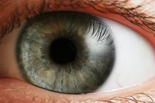
To better understand this problem, I am going to step through the parts of this statement and explain what I mean by each. First, I mention that the imaging problem involves the use of an optical system. I have to admit that I use this term partly because it is part of the jargon of the optical sciences, but I also think that the word "system" nicely captures the essence of what I would like to say. An optical system is a collection of components such as lenses, mirrors, and prisms taken together with their mechanical supports and arranged in a meaningful way to capture and channel light as it travels from one place to another. Below is one example of an optical system that most people know pretty well.

A human eye is an optical system! From http://en.wikipedia.org/wiki/Eye#/media/File:Eye_iris.jpg, Peter Nóvak, Wikipedia.

I have already mentioned that the components of an optical system can include things we commonly associate with optics, such as lenses and mirrors, but really no one such component is necessary to build an optical system so long as it captures and does something with light. For example, the pinhole camera uses nothing but a very small hole to form images; no lens is required! Still, we usually find some components like lenses much more frequently in optical systems than others, and the choice of which components to use really just depends on the specific type of imaging problem you are trying to solve.

Next in the statement of the imaging problem I say that we will be forming an image by arranging the components of our optical system in a clever way. Though the intuitive notion of an image is quite clear, I think it is actually extremely difficult to formally define it. For the purpose of this tutorial, I think it is best at this point to rely on the intuitive idea of an image until I have developed enough concepts to define it in terms of optical theory [2].

Finally, the imaging problem involves determining the location, size, and orientation of an image formed by the system. This means that rearrangement of our system's components is going to change these features of the image. Things such as the size of a CCD chip or the weight of a lens are going to place constraints on the values these properties can take.

Perfect imaging systems

At this point I should stress that paraxial optics is not the only theoretical tool for solving the imaging problem. We clearly can use non-paraxial geometrical optics or wave optics to determine the properties of an image formed by an optical system. However, what is interesting is that paraxial optics is one of very few theoretical frameworks in which a perfect image can be realized [3].

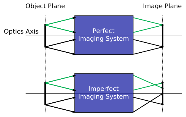
Perfect optical system

The above figure, which is called a ray-trace diagram, illustrates what I mean by a perfect imaging system. The system is represented as a "black box" that collects light coming from a two-dimensional plane (known as the object plane) and relays the light to another plane known as the image plane. The whole system is considered to be rotationally symmetric about a line called the optics axis so that I can represent it as a two-dimensional sketch instead of requiring a full, three-dimensional model. Finally, light is modeled as lines with arrows denoting the direction of propagation [4].

Now comes the important point. Within the framework of paraxial optics theory, it is possible to show that, given an object plane and an image plane, one can construct an optical system consisting of components that redirect the light rays in such a way that all the rays leaving a point in the object plane are brought back together at a corresponding point in the image plane. This means that the perfect optical system performs a one-to-one mapping of points in the object plane to points in the image plane. What's more, the distance between every point in the image plane and the optics axis is proportional to the distance between their corresponding points and the axis in the object plane by a constant factor. This factor is known as the magnification of the system.

The way this perfect imaging system is realized within the context of the theory is in the way the components redirect the rays coming from the object [5]. What differentiates /paraxial/ geometrical optics from plain old geometrical optics is the rules dictating how the redirection occurs.

One other important point is to consider what happens in imperfect imaging systems. Once we violate the assumptions of paraxial optics so that we no longer have a system operating within its range of validity, we cannot perform a true, one-to-one mapping of points from the object plane to the image plane. Instead, we find that rays coming from a single point in the object plane cannot all be brought back together in any image plane [6]. We could say that the image plane is a concept that does not exist outside paraxial optics. And if the image plane does not exist, how are we to strictly define an image size and location?

Of course, we can find planes in non-paraxial systems in which there are pretty good images, and these usually correspond to the image planes we find by applying the equations and simplifications of paraxial optics. So paraxial optics is often our first tool for modeling an imaging system. It tells us roughly where our images will be formed and how big they are, but it will not tell us about image quality.

Conclusion

With this tutorial I hope to have provided you with a conceptual basis for understanding paraxial geometrical optics without including too many of its details. I think a conceptual basis such as this is much better than diving right into ray-trace diagrams with lenses and mirros. I think new students to optics often wonder what the importance is of paraxial optics and why it is needed when more complete optical descriptions exist. I hope that the discussion of the perfect imaging system and its existence only within the framework of paraxial geometrical optics helped to clarify its importance.

Footnotes

  1. You didn't expect me to give you the answer right away, didyou? :)
  2. Even the Wikipedia entry on the concept of an Image is a bit vague and philosophical.
  3. Maxwell's Fisheye lens is another, but it is a good deal more complicated and, to my knowledge, has not been demonstrated at optical wavelengths.
  4. It's important to realize that we are modeling the propagation of light as a ray; we are not saying that light is a ray. If light really was a ray and not an electromagnetic wave, then we would not need the wave theory of optics to explain phenomena like diffraction. Within the framework of the axioms of geometrical optics, a ray adequately describes how light propagates.
  5. More specifically, it lies in the linearization of Snell's law, but I won't get into that yet.
  6. This phenomenon is precisely what an optical aberration is within geometrical optics theory.

Can my laser beam be collimated?

The fluorescence microscopy setup in my lab requires quite a bit of power. The minimum irradiance requirement is greater than 1 kW per square centimeter, and this must cover an area spanning a few tens of microns across after focusing through the objective. When I was designing the setup, the highest priority was placed on finding a cheap laser with as much power as possible at a wavelength of 647 nm; I considered all other qualities of the laser of secondary importance.

Just like everything else in science, I have learned a very good lesson from this experience. The laser I decided to purchase is a 800 mW BrixX laser from Omicron. The cost is under $10,000, which I consider to be a pretty good deal for the amount of power it puts out. There is no fiber-coupled version, but all of our lasers are free space anyway so I did not consider this to be a big problem. The beam is astigmatic, which is to be expected from a high power laser diode.

The astigmatism is not necessarily a big problem for me, though. What is surprising to me is how difficult it is to keep the beam collimated over large distances, that is, to keep it roughly the same size as it propagates. My application requires a fairly small beam size since the exit pupil of the objective is only 6 millimeters in diameter. With M-squared values direct from the laser of 12 and 25, it is quite difficult to keep the beam collimated for a long enough distance to steer the beam through all the optics and to keep it small enough to prevent overfilling the objective's exit pupil and losing power.

What I have learned from this is that free-space diode lasers, and more generally multimode laser beams, require extra consideration to ensure that they will stay collimated in long setups.

So, how can I predict the distance over which my beam can stay collimated to better judge how well it will work for my setup? The first thing to realize is that no beam can stay collimated forever. Real laser beams experience diffraction, which causes them to spread as they propagate. This means that the first thing I should do is to consider the distances spanned by the beam paths. In a microscopy setup, this path will probably not be longer than a couple meters. In mine, it's roughly two meters since I am combining a number of laser beams together and need the extra space.

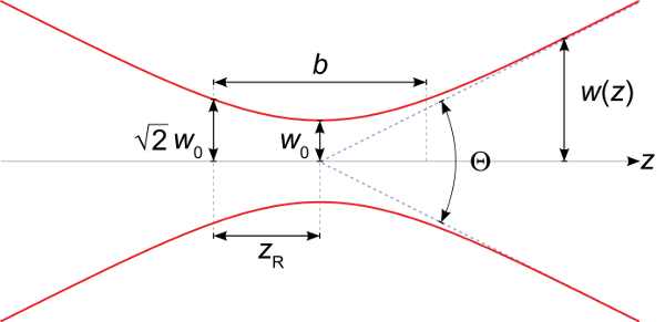
Once I identify the length scale over which the beam should stay collimated, I need to examine the beam parameter that is best associated with collimation. For a pure Gaussian beam, this parameter is the Rayleigh range. The Rayleigh range is the distance between the beam waist and the point where the cross-sectional area of the beam has doubled, or, equivalently, to the point where the radius of the beam has increased over the waist radius by a factor of the \(\sqrt{2}\). For a pure Gaussian beam with a waist radius of \(w_0\) and a wavelength of \(\lambda\), the Rayleigh range is given by the equation

\begin{equation*} z_R = \frac{\pi w_0^2}{\lambda} \end{equation*}

It is represented by the symbol \(z_R\) in the figure below from Wikipedia. The total distance over which the beam will stay collimated is represented by \(b\) and is just twice the Rayleigh range.

Gaussian beam waist

The Rayleigh range of a Gaussian laser beam should therefore be larger than the characteristic distance of my setup that I identified in the previous step. But what about multimode beams like the one from my laser diode? This is where the concept of an "embedded Gaussian" comes into play. (For more information about this idea, see this tutorial by Tony Siegman.) I can predict the collimated distance by computing the Rayleigh range of an ideal Gaussian beam, and then divide it by the \(M^2\) parameter for the beam.

Let's take an example using numbers from my own laser. I will first pretend there are no collimating optics in the laser, which is not true but will serve as a good example as to why diode lasers without collimating optics are not good for free space setups. From the laser's spec sheet, I know that the \(M^2\) value in the bad direction is 25 and that its waist size, which is probably half the size of the diode in one principle direction, is 107 microns. Using the above equation, I get a value of 56 centimeters, which means that an ideal Gaussian beam with these specs will stay collimated over about half a meter.

However, my real multimode beam will have a Rayleigh range that is smaller than this value by a factor of 25, which is only about 2 centimeters. For this reason, diode laser beams almost always have collimating optics; the beam from the diode itself is highly divergent.

Returning to my own setup, if I resize the beam using a telescope to have a waist radius of 2 millimeters so it almost entirely fits inside the objective's exit pupil, the Rayleigh range of the embedded Gaussian beam will be almost 20 meters, which is pretty long. The real beam, however, will have a Rayleigh range of about 780 millimeters meters due to the high \(M^2\) value. Practically, this means I have about one meter of collimated laser beam with which to work since I have double the Rayleigh range of collimated distance, but really I want the beam to travel less distance than this.

Fortunately I can shrink the beam path enough that this should not be a problem, but it does serve as a very good lesson when looking for lasers for a microscopy application.

Relearning paraxial optics

As a microscopist who designs and builds custom microscopes, I often find that first order ray tracing is one of the most useful tools I have. It is most useful to me when I am starting a design or for checking that I have not made any serious logical blunders when working at the bench. I also find it to be a good teaching tool and excellent for communicating my designs to others.

Since I have recently made a lot of back-of-the-envelope ray trace designs for a microscope I am building at work, I have begun to critically think about why ray tracing works so well and how it fits inside the structure of the physical theories of optics.

Ray tracing is a technique derived from paraxial geometrical optics and really is just a consequence of the axioms and assumptions in the development of the theory. When I think back to when I first learned about paraxial optics, however, I am reminded of severe assumptions that place limits on the scope of its validity. So how can a theory that makes such an enormous simplification by treating the electromagnetic waves described by Maxwell's equations as lines obeying the rules of geometry still be so useful?

In this next series of blog posts, I want to explore this question and take the time to relearn paraxial optics with the benefit of hindsight. Physicists typically learn paraxial optics as their first theory of optics because it is relatively easy as compared to electromagnetism and quantum optics. I am curious what aspects of the theory I can appreciate now that I am familiar with the more advanced optical theories.

The picture below might also provide a bit of motivation for why this interests me: we physicists learn about optics theories in a direction of increasing complexity during our education. However, this approach also means that we learn the most general theories last, so it is not obvious why assumptions and approximations are made in the theories we learn first. The result, I think, leads to a bit of logical discordance in our minds that can prevent a clear understanding of the subject. With this series of posts I hope to remove this cognitive dissonance and improve my understanding of the field I work in.

The order of optics theories

Reading select lines from a text file

I just created a Python Gist for reading select lines from a text file into memory. I came up with this Gist when I needed to parse the core log from our microscope control software (Micro-Manager). One of our devices was continously sending its statistics to the computer, which would then be recorded to the log. I wanted to find only lines that contained the statistics by searching for the STATS identifier, which was unique to these lines.

The problem was a bit more difficult than reading just the lines containing this string because I wanted the statistics only for times when the software was acquiring a time series of images. Luckily, the core log also contains lines with unique strings indicating when a time series was initiated and stopped. All lines in the log are time-stamped.

Below is the Gist I used to solve this problem. The lines that will be retained in memory will contain the strings in the list lineFilters. I then define a function named stringIsIn that will return a list of bool indicating whether each string is present in the line.

At the bottom of the Gist, I use a list comprehension to loop over each line in the file. The line is appended to a growing list called outputLines if the line contains any of the strings I defined. Note that it's not necessary to use a separate definition for stringIsIn; the list comprehension over lineFilters could have been placed inline with the primary list comprension over lines in the file. I do think it is more readable the way it is presented below, however.

I welcome any comments or suggestions, especially on the Gist website where others may be more likely to find it.

filename    = 'myFile.txt'
outputLines = []

# Keep all lines containing ANY of the following list of strings.
lineFilters = ['line 1',
               'line 2',
               'line 3']
stringIsIn  = lambda line: [filter in line for filter in lineFilters]


# Read only lines containing one of the strings into memory.
with open(filename, 'r') as file:
    [outputLines.append(line) for line in file if any(stringIsIn(line))]

The basics of virtualenv

I use Python 3.4 in most of my data analyses and in some simulations. I like a lot of its features, like its implementation of generators, maps, and filters. However, much of the software on my Debian Wheezy system depends on Python 2.7 to run, such as Mendeley. (It used to run just fine with Python 3.4, until I ran an automatic update and that was the end of that.)

To run some Python 2.7 programs, I used to do the following:

sudo rm /usr/bin/python
sudo ln -s /usr/bin/python2.7 /usr/bin/python

I know. Ouch. Every single time I needed to run a program that depended on python2.7, I would delete the symlink in /usr/bin, make a new link to python2.7, and then run my program. When I needed to give various programs convenient access to python3.4, I would delete the symlink and create a new one to the newer version.

This was dumb, because there is a convenient Python-based tool that can fix the problem of needing multiple versions of Python (and libraries!) on the same system. The solution to this problem is called virtualenv.

There are a lot of descriptions about what virtualenv is on the internet, so I won't bother going into details here. Instead, I will focus on just the very basics of its setup and use so that I can have a handy future reference for when I forget how something works and so that others can profit from what I have learned. Most everything I've done came from python-guide.org, so I'm more-or-less putting what they have already said into my own words.

To start, I already have Python 2.7 and 3.4 installed on my system. In principle, you do not need them installed at the system level, but I already have done this so I will start from there. I first installed pip for Python 2.7 since I only had pip3 on my system to start. I did this because I want to keep Python 2.7 as my system's default Python environment.

sudo apt-get update
sudo apt-get install python-pip

Once installed, I used it to install virtualenv and virtualenvwrapper. The latter provides some nice features for working with virtualenv.

sudo pip install virtualenv
sudo pip install virtualenvwrapper

Now, virtualenvwrapper requires an environment variable to tell it where to store the folders for each virtual environment. This environment variable is called WORKON_HOME. First, I created the folder it will point to:

mkdir ~/Envs

Next, I edited my ~/.bashrc and added the following line:

export WORKON_HOME=~/Envs

All of my virtual environment files (except for the Python intepreters) will be stored in this folder. Finally, I restarted my terminal window so that the environment variable was assigned. You can check this by typing =echo $WORKON_HOME= in your new terminal window. If it returns the path to your new environments folder, then you should be fine.

Next, I ran the virtualwrapper setup script. Note that I did not need sudo (in fact, sudo could not find a command called source) and that no output is returned when the script is run.

source /usr/local/bin/virtualenvwrapper.sh

Now virtualenvwrapper should be installed, so let's make a virtual environment. We can do this using the mkvirtualenv command, followed by a name for the environment. I will use the name venv in this example, like Kenneth Reitz did in his guide that I linked above.

mkvirtualenv venv

To start the new virtual environment, type workon venv and note that change in the prompt, indicating which environment you are in. You now have a fresh Python environment to which you can add any library you wish. To leave the environment, type deactivate into your terminal.

One simple test that you can do to see whether your Python environment really is clean is to run the Python interpreter from inside your environment and try importing a module that you know is in your system-wide site packages but not in your virtual environment. For example, inside venv I type =python= at the terminal prompt and tried importing numpy, which I had not yet installed in venv:

import numpy

This returned an ImportError: No module named numpy. Since I do have numpy installed on my system but not in this environment, it tells me that the environment is likely clean.

To install new libraries, simply use pip or install them to the folder that was created for this environment in ~/Env. To delete a virtual environment entirely, use rmvirtual env.

Now, how can I specify that I want the virtual environment to use the python3.4 interpreter in a virtual environment named python3-general? Doing so would solve my original problem. Simply make a new virtual environment like so:

mkvirtualenv -p /usr/bin/python3.4 python3-general

Voilà. C'est tout. I hope this helps you get up and running with this great tool!