Accessing the Raspberry Pi camera image sensor

WARNING You can easily ruin your Raspberry Pi camera module by following the steps in this post. Proceed with caution.

Over the past half year I have been making slow but steady progress on my lensless imager project. The purpose, aside from having a bit of fun, is to create an imaging system for basic cell biology that doesn't use an expensive microscope objective.

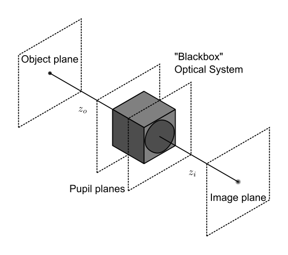
A lensless imager works just as its name implies: an image sensor records the scattered light from a microscopic, transparent object and computationally reconstructs an image of that object, all without a lens. The best resolutions are achieved when the object is relatively close to the image sensor. Ideally, the separation between the object and the sensor's pixels would be at most about one millimeter. This limit is partly determined by the light source's spatial coherence, but also by the fact that high resolution is achieved by recording the scattered light at very large angles, which is possible only when the sample is close to the sensor.

Today I had a bit of free time so I decided to see whether I could remove the housing that surrounds the Raspberry Pi camera's sensor. The Raspberry Pi Camera Module version 2 sensor is a Sony IMX219 color chip. Directly above the sensor is a filter, a lens, and the housing for both of these that prevent me from placing anything closer than about half a centimeter from the sensor plane. If I would want to use this camera for the lensless imager, then the housing would have to go.

Now, even without the housing the Raspberry Pi camera is not necessarily the best option for the project because the IMX219 is a color sensor. This means that there is a Bayer filter over its pixels, which would cut the resolution of the imager since I would be using a very narrow band light source. Effectively, only a quarter of the pixels would be receiving any light. Regardless, I had a spare second camera and it interfaces well with the Raspberry Pi, so I figured it would make for a good prototype.

As you will see, I did slightly damage my sensor, though it seems to still work. You can easily ruin your camera module or cut your finger by following these steps, so proceed at your own risk.

Step 0: The Raspberry Pi Camera Module V2

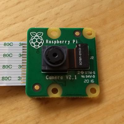
In the picture below you see my Raspberry Pi Camera Module. From above, you can see the small circular aperture with the lens immediately behind it. The sensor is inside the small gray rectangular housing that is attached to the control board by a small ribbon cable (to its right) and a bit of two-sided sticky foam tape (underneath the sensor; not visible).

The Raspberry Pi Camera Module V2

Step 1: Remove the main ribbon cable

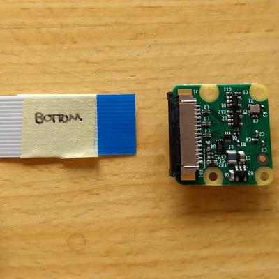
To make working on the board a bit easier, I removed the white ribbon cable that attaches the module to the Pi. I did this by pulling on the black tabs on the two ends of the connecter until the cable is easily removed. I labeled the sides of the ribbon cable just in case.

Remove the main ribbon cable from the control board

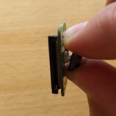
Step 2: Detach the sensor's ribbon cable

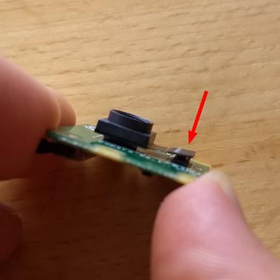
Next, I used my finger and thumb nail to remove the small ribbon cable that attaches the sensor to the control board. I essentially applied a small torque to the bottom edge of the connector until it just "popped" up, as seen in the second image below.

The small ribbon cable from the sensor is to the right.

Step 3: Remove the sensor from the control board

In the third step, I used my thumbnail to gently pry the sensor from the control board. The sensor is attached with some two-sided sticky tape and may need a few minutes of work to come free.

Pull the sensor off the control board.

Step 4: Remove the rectangular housing

In this step you risk cutting your finger, so please be careful.

The housing around the sensor is glued. To remove it, you will need to gently work a knife (or, better yet, a thin screw driver) between the housing and the sensor board, taking care not to let the blade go too far into the housing and possibly ruining one of the resistors or wire bonds.

Cut carefully on one side of the housing.

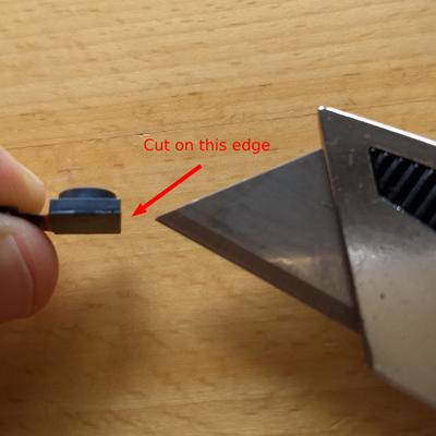
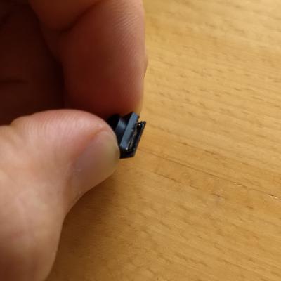
Once you get a knife between the two, try popping the housing off of the sensor.

Once the edge is cut, pop the housing off.

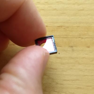
When I did this I cut on three sides of the housing, but in retrospect I should have only cut on the side opposite the ribbon cable and pried the other sides loose. This is because I damaged a small resistor when the knife blade went too far into the housing. You can see this below and, at the same time, get an idea of the layout of the sensor board so you know where you can and can't cut.

The resistor near the top of the board was damaged when cutting the housing.

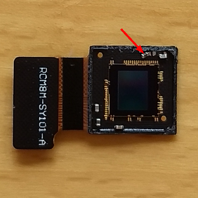
If you have the normal version of the camera, then you can also find the IR blocking filter inside the housing.

The IR blocking filter.

Fortunately for me the camera still works, despite the damaged resistor. I can now place samples directly on the sensor if I wanted to, though the wire bonds from the sensor to its control board appear quite fragile. For this reason, it may make more sense to build a slide holder that holds a sample just above the surface without touching it. For now, I can use this exposed sensor to prototype different methods for mounting the sample.

Modeling noise for image simulations

In my previous post, I described a method for simulating inline holography images. The ultimate purpose of doing this was to generate holography data that could be used to test the performance of different reconstruction algorithms. Since I would know the input object, I could apply the reconstruction algorithm to the holograms and see how closely the reconstructed object matched the known input.

My modeling however ignored an important aspect about the holographic process, namely the acquisition of digital images and the assoicated noise that would accompany the raw data. This is important because holographic reconstruction algorithms need to be robust against the uncertainty that will inevitably be introduced by recording the hologram with a digital camera.

In [1]:
%pylab inline
import scipy
from numpy.fft import fft2, fftshift, ifftshift
from mpl_toolkits.axes_grid1 import make_axes_locatable
from matplotlib import animation
plt.style.use('dark_background')
plt.rcParams['figure.facecolor'] = '#272b30'
plt.rcParams['image.cmap'] = 'viridis' 

print('Python version:\n{}\n'.format(sys.version))
print('Numpy version:\t\t{}'.format(np.__version__))
print('matplotlib version:\t{}'.format(matplotlib.__version__))
print('Scipy version:\t\t{}'.format(scipy.__version__))
Populating the interactive namespace from numpy and matplotlib
Python version:
3.7.0 (default, Aug 17 2018, 19:20:07) 
[GCC 5.4.0 20160609]

Numpy version:		1.16.1
matplotlib version:	3.0.2
Scipy version:		1.2.1

A Mathematical Model for Camera Noise

One of the best descriptions of camera noise that I have ever found may be the EMVA 1288 Standard. This document details a standard set of models and procedures to characterize CMOS and CCD cameras and light sensors. From its website:

EMVA launched the initiative to define a unified method to measure, compute and present specification parameters for cameras and image sensors used for machine vision applications... [The EMVA Standard] creates transparency by defining reliable and exact measurement procedures as well as data presentation guidelines and makes the comparison of cameras and image sensors much easier.

In particular, chapters 2 and 3 of the Standard provide a very clear and concise description the mathematical model for CCD/CMOS camera noise. Below, I have adapted the image of the mathematical model presented at the beginning of chapter 2.

Optical system with pupils

In this model, the camera/sensor is a single pixel that takes an input (a number of photons) and transforms this number to an output (a digital value in analog-to-digital units, or ADU). In performing this transformation, various sources of noise are added to the signal so that, given a camera's output in ADU, we can only make probabilisitic inferences about the actual number of photons impinging upon it. There are also a few assumptions in this model that, when taken together, constitute what's called an ideal image sensor. They are:

  1. the numer of photons collected by the pixel depends on the product of irradiance $ E \, \left[ W / m^2 \right] $ and the exposure time $ t_{exp} \, \left[ s \right] $;
  2. the sensor is linear, i.e. the digital signal $ y $ increases linearly with the number of photons received;
  3. all noise sources are constant in time and space;
  4. only the total quantum efficiency of the camera is dependent on the wavelength of the incident irradiation;
  5. and only the dark current depends on the temperature.

From these five assumptions, the laws of quantum mechanics, and the laws of probability, expressions for the mean output, $ \mu_y $, the variance of the output $ \sigma_y^2 $, and the signal-to-noise ratio ($SNR $) may be derived.

\begin{equation*} \mu_y = K \mu_d + K \eta \mu_p \\ \sigma_y^2 = K^2 \sigma_d^2 + K \left( \mu_y - K \mu_d \right) \\ SNR = \frac{\eta \mu_p}{\sqrt{\sigma_d^2 + \sigma_q^2/K^2 + \eta \mu_p}} \end{equation*}

In these expressions, $\mu$ and $\sigma^2$ represent the mean and variance of the number of photons hitting the camera ($p$), the dark noise ($d$), and the output signal in ADU's ($y$). The number of electrons $ \mu_e $ generated by $\mu_p$ photons hitting the active area of the sensor is obtained from the expression for the quantum efficiency $\eta$, an engineered property of the camera that in general depends on the wavelength.

\begin{equation*} \eta \left( \lambda \right) = \frac{\mu_e}{\mu_p} \end{equation*}

The sensitivity of the camera $K \, \left[ ADU / e^- \right] $ represents the amplification of the voltage in the pixel from the photoelectrons and is also a property of the camera. Finally, $ \sigma_q^2 $ represents the noise introduced by digitzing the continous voltage signal into a digital one.

The EMVA 1288 Standard explains how to derive these expressions from the assumptions and known physical laws, so I will not go into their derivations in this post. Instead, I will focus on explaining how we can use this model to simulate the effects of camera noise in our holograms.

From Model to Simulation

The goal of the simulation will be to take a simulated hologram as input and convert it into an image that might be captured by a digital camera. This means that the final image should contain noise that is realistic and follows the rules of the model.

The model will depend on five free parameters that vary from camera-to-camera. They are:

  1. the total quantum efficiency $ \eta $;
  2. the read noise variance $ \sigma_{r}^2 $ (or its standard deviation);
  3. the dark current $ \mu_I $;
  4. the sensitivity $K$;
  5. and the bit-depth of the camera $k$.

The dark noise $ \sigma_d^2 $ is actually comprised of two separate noise sources, i.e. the read noise $ \sigma_r^2 $ and the dark current $ \mu_I $. Because the noise sources are independent, we can write

\begin{equation*} \sigma_d^2 = \sigma_r^2 + \sigma_I^2 \\ \sigma_d^2 = \sigma_r^2 + \mu_I t_{exp} \end{equation*}

where the last step relies on the fact that the generation of thermal electrons is a Poisson process whose mean is equal to its variance. The units of $\mu_I$ are $e^- / s $ and values for $ \mu_I $ are often provided on camera spec. sheets. Likewise, the read noise $\sigma_r^2$ is also provided on spec. sheets, although in my experience the units are likely to be in root-mean-square electrons or median electrons and not electrons-squared.

Other than the inputs, we do not need to provide values for the other numbers in the model because they are related to the free parameters by various physical and mathematical laws.

Finally, let's ignore spatial noise sources in these simulations because it's difficult to characterize them with a single number. Spatial noise is a variation in the free parameters of the camera from pixel to pixel. An example of a common type of spatial noise is photon response non-uniformity and is manifest in a sensitivity $ K $ that varies between pixels. Ignoring spatial noise in the simulations simply means that values for the read noise, dark current, quantum efficiency, and sensitivty are the same for all pixels.

Step 0: Convert the electric field to photons

Before doing anything, we need to take the electric field from our Fourier optics simulations and convert it to units of photons. If it isn't clear how you would first get an electric field, you can refer to my previous post on calculating the hologram of a thin, circular phase-only object. Typically, the calcuation of the electric field will follow from the laws of diffraction and serve as an input for the camera model.

To get the number of photons, we first compute the irradiance of the field using the magnitude of the time-averaged Poynting vector of a linearly-polarzed electromagnetic wave in free space, which is

\begin{equation*} E \left(x, y \right) = \frac{1}{2Z_o} \left| U\left(x, y \right) \right|^2 \end{equation*}

Here, $E \left( x, y \right) $ is the irradiance at point $ \left( x, y \right) $, $U \left( x, y \right) $ is the scalar electric field at the same point, and $Z_0 = 377 \, \Omega $ is the impedance of free space. We would change the value for the impedance if we were imaging in a medium other than vacuum. The units of the field are $ V / m $ which, when squared and divided by the units of the impedance (Ohms), gives units of power per area, or $ W / m^2 $. It's also worth mentioning that we are implicitly assuming the field varies smoothly on the length scale of a pixel. This is why we can use the expression for the Poynting vector of a plane wave.

The mean number of photons is obtained from the irradiance by the expression

\begin{align*} \mu_p &= \frac{\lambda A}{hc}Et_{exp} \\ &= \frac{\lambda A}{2hcZ_0} \left| U \right|^2 t_{exp} \end{align*}

where $ A $ is the pixel's area and $ \frac{hc}{\lambda} $ is the energy per photon in units of Joules, with $hc = 2 \times 10^{-25} \, J \cdot m $.

This step is a bit cumbersome, and in the rest of what follows I will skip this step and will use a set number of photons directly as the input to the simulations, rather than a scalar field.

Step 1: Compute the photon shot noise

For the sake of simplicity, let's start by assuming that we have a camera with $ 256 \times 256 $ pixels and a mean incident photon flux of 500 photons on each pixel. This would produce an image that looks like this:

In [2]:
num_photons = 500
num_pixels  = 256
mu_p        = num_photons * np.ones((num_pixels, num_pixels))

fig, ax = plt.subplots()
img = ax.imshow(mu_p, vmin=400, vmax=600)
ax.set_xticks([])
ax.set_yticks([])
ax.set_title('No noise')

cb = plt.colorbar(img)
cb.set_label('Photons')

plt.show()

Photon shot noise arises from the fact that the incident number of photons is not deterministic but rather a random process whose statistics are Poissonian. In a Poisson process, the variance of the noise $ \sigma_p^2 $ is equal to the mean number of photons $ \mu_p $.

Poisson random numbers are easy to generate with NumPy. First, we set a seed so that we can reproducibly generate the same random numbers each time and initialize a RandomState instance with it. Using this RandomState instance, we call the poisson method with a mean of num_photons and a size (num_pixels, num_pixels). Finally, we plot the image and compare it to the one where no shot noise is present.

In [3]:
seed       = 42
rs         = np.random.RandomState(seed)
shot_noise = rs.poisson(num_photons, (num_pixels, num_pixels))

fig, (ax0, ax1) = plt.subplots(ncols=2)
img0 = ax0.imshow(mu_p, vmin=400, vmax=600)
ax0.set_xticks([])
ax0.set_yticks([])
ax0.set_title('No shot noise')

divider = make_axes_locatable(ax0)
cax = divider.append_axes("right", size="5%", pad=0.05)
cb0 = plt.colorbar(img0, cax=cax)
cb0.set_ticks([])

img1 = ax1.imshow(shot_noise, vmin=400, vmax=600)
ax1.set_xticks([])
ax1.set_yticks([])
ax1.set_title('Shot noise')

divider = make_axes_locatable(ax1)
cax = divider.append_axes("right", size="5%", pad=0.05)
cb1 = plt.colorbar(img1, cax=cax)
cb1.set_label('Photons')

plt.show()
In [4]:
# It's also interesting to look at the distribution of photons hitting each pixel.
plt.hist(shot_noise.ravel(), bins=np.arange(350, 650))
plt.xlabel('Number of photons per pixel')
plt.ylabel('Frequency')
plt.show()

Step 2: Compute the number of photoelectrons

At this point we're going to need some numbers for our camera. For this example, I chose a camera using the popular Sony IMX264 CMOS chip, the FLIR Chamleon 3 (part number CM3-U3-50S5M-CS). Here are some of the key specs for our modeling:

Spec Value
Quantum efficiency (at 525 nm) 0.69
Sensitivity 5.88 ADU / e-
Temporal dark noise 2.29 e-
Pixel size 3.45 microns
Analog-to-digital converter (ADC) 12-bit

Assuming our light has a wavelength of 525 nm, then the number of photoelectrons is simply the product of the quantum efficiency with the realization of the field.

In [5]:
quantum_efficiency = 0.69
# Round the result to ensure that we have a discrete number of electrons
electrons = np.round(quantum_efficiency * shot_noise)

fig, (ax0, ax1) = plt.subplots(ncols=2)
img0 = ax0.imshow(shot_noise, vmin=200, vmax=600)
ax0.set_xticks([])
ax0.set_yticks([])
ax0.set_title('Photons')

divider = make_axes_locatable(ax0)
cax = divider.append_axes("right", size="5%", pad=0.05)
cb0 = plt.colorbar(img0, cax=cax)
cb0.set_ticks([])

img1 = ax1.imshow(electrons, vmin=200, vmax=600)
ax1.set_xticks([])
ax1.set_yticks([])
ax1.set_title('Electrons')

divider = make_axes_locatable(ax1)
cax = divider.append_axes("right", size="5%", pad=0.05)
cb = plt.colorbar(img1, cax=cax)

plt.show()

Step 3: Simulate read noise and dark current

Following the schematic of the camera model above, we see that we next need to add the dark noise. Dark noise (not to be confused with dark current) refers to the noise in the pixels when there is no light on the camera. Typically we deal with two sources of dark noise: readout (or just "read") noise and dark current. The camera specs in our example only provide us with the total dark noise, which is not surprising since dark current is not very significant in microscopy or machine vision. (It is however significant in astronomy because of the very long exposure times of several seconds or more, which allows appreciable dark current electrons to accumulate during the exposure.)

To the best of my knowledge, when dark noise is primarily read noise we may well model it as a Gaussian distribution whose standard deviation is equivalent to the dark noise spec of the camera. This modeling approach is taken, for example, in the 2016 SMLMS Challenge, a community-driven competition to identify the best reconstruction algorithms for single molecule localization microscopy. Please note that the noise model employed in the challenge was for an electron multiplying CCD (EMCCD), so you may find that it differs slightly from what I am discussing here.

In [6]:
dark_noise = 2.29 # electrons
electrons_out = np.round(rs.normal(scale=dark_noise, size=electrons.shape) + electrons)

fig, (ax0, ax1) = plt.subplots(ncols=2)
img0 = ax0.imshow(electrons, vmin=250, vmax=450)
ax0.set_xticks([])
ax0.set_yticks([])
ax0.set_title('Electrons In')

divider = make_axes_locatable(ax0)
cax = divider.append_axes("right", size="5%", pad=0.05)
cb0 = plt.colorbar(img0, cax=cax)
cb0.set_ticks([])

img1 = ax1.imshow(electrons_out, vmin=250, vmax=450)
ax1.set_xticks([])
ax1.set_yticks([])
ax1.set_title('Electrons Out')

divider = make_axes_locatable(ax1)
cax = divider.append_axes("right", size="5%", pad=0.05)
cb = plt.colorbar(img1, cax=cax)
cb.set_label('Electrons')

plt.show()
In [7]:
# Plot the difference between the two
fig, ax = plt.subplots()
img = ax.imshow(electrons - electrons_out, vmin=-10, vmax=10)
ax.set_xticks([])
ax.set_yticks([])
ax.set_title('Difference')

cb = plt.colorbar(img)
cb.set_label('Electrons')

plt.show()

Step 4: Convert from $ e^- $ to ADU

Now we need to convert the value of each pixel from electrons to ADU, or analog-to-digital units. ADU's are the units of grey scale that are output by monochrome cameras. To do this, we multiply the number of electrons after the addition of read noise by the sensitivity. We also need to ensure that the final ADU count is discrete and to set the maximum upper value of ADU's to the $ 2^k - 1 $ where $ k $ is the camera's bit-depth. The latter operation ensures that saturation of the pixels is correctly modeled.

In [8]:
sensitivity = 5.88 # ADU/e-
bitdepth    = 12
max_adu     = np.int(2**bitdepth - 1)
adu         = (electrons_out * sensitivity).astype(np.int)
adu[adu > max_adu] = max_adu # models pixel saturation

fig, ax = plt.subplots()
img = ax.imshow(adu)
ax.set_xticks([])
ax.set_yticks([])

cb = plt.colorbar(img)
cb.set_label('ADU')

plt.show()

Step 5: Add a basline

Many cameras have a built-in baseline ADU value. This prevents the number of ADU's from becoming negative at low input signal. The Andor Zyla 4.2, for example, has a baseline value of 100 ADU. If you take a large number of dark frames and compute the average of each pixel in a Zyla, the average values will very nearly be 100.

We don't have baseline information for this camera, but 100 seems like a reasonable assumption. Here's what our final image will look like if we had a constant average of 500 photons incident on each pixel.

In [9]:
baseline  = 100 # ADU
adu      += baseline

# EDIT: Note that we could have easily just performed this next step once
# here, rather than in the previous step
adu[adu > max_adu] = max_adu


fig, ax = plt.subplots()
img = ax.imshow(adu)
ax.set_xticks([])
ax.set_yticks([])

cb = plt.colorbar(img)
cb.set_label('ADU')

plt.show()

Adding noise to a simulated hologram

Let's see how the hologram from my last post will look like if I add camera noise to it. I'm going to assume that we are using the same camera as in my example to record the hologram. First, we'll setup the Fourier optics code as before to make the hologram. Then, we'll write a function that adds the noise and, in each frame of the animation, call it with the calculated field as an input.

This first part more-or-less repeats the essential bits of my last post. We make a circular object that doesn't absorb any light but which has a refractive index which causes a constant phase shift of 0.75 radians. We then use Fourier optics to compute the scattered field in the same plane as the object; this will be the starting frame of the animation. Instead of directly computing the number of photons per pixel from the field, we simply renormalize it so that the maximum value is 100 photons. 100 photons might seem like a weak signal, but this is actually quite a good camera and we will need to make the signal weak so that we can see the noise in the movie. In fact, the spec sheet for the camera reports an absolute minimum detectable signal of about 4 photons per pixel.

In [10]:
# Ground truth: a circular phase-only object
numPixels = 512
gtRadius  = 50 # ground truth radius, pixels
gtPhase   = 0.75 # radians
gtCenter  = numPixels / 2 # assumes numPixels is even
W, H      = np.meshgrid(np.arange(0, numPixels), np.arange(0, numPixels)) # coordinates of the array indexes
gtMask    = np.sqrt((W - gtCenter)**2 + (H - gtCenter)**2) <= gtRadius # boundaries of the object
gt = np.ones((numPixels, numPixels), dtype=np.complex)
gt[gtMask] = np.exp(1j * gtPhase)

# Physical dimensions and sampling
pixelSize = 0.1 # microns
x = np.linspace(-pixelSize * numPixels / 2, pixelSize * numPixels / 2, num = numPixels, endpoint = True)

dx = x[1] - x[0]    # Sampling period, microns
fS = 1 / dx         # Spatial sampling frequency, inverse microns
df = fS / numPixels # Spacing between discrete frequency coordinates, inverse microns
fx = np.arange(-fS / 2, fS / 2, step = df) # Spatial frequency, inverse microns

# Fourier transform of ground truth
GT = ifftshift(fft2(fftshift(gt))) * dx**2

# Angular spectrum propagator and spatial frequencies
def H(fx, fy, z, wavelength=0.5):
    square_root = np.sqrt(1 - (wavelength**2 * fx**2) - (wavelength**2 * fy**2))
    temp = exp(1j * 2 * np.pi * z / wavelength * square_root)
    temp[np.isnan(temp)] = 0 # replace nan's with zeros
    return temp

FX, FY = np.meshgrid(fx, fx)

# Field at a distance of z=0
gt_prime = fftshift(ifft2(ifftshift(GT))) / dx**2

# Normalizing constant: makes the maximum photon count at z = 0 equal to 100 photons
norm = np.max(np.abs(gt_prime)**2) / 100

Next we create a Python function which takes as input a map of photons per pixel from our Fourier optics calculations and our camera specs. Since it doesn't have a large effect, I am skipping the explicit rounding of continuous numbers at each step and saving it until the end when the ADU's are calculated. I also added a random number generator to the inputs in case you want to reproduce previous results, but this isn't too important for this post.

In [11]:
# Function to add camera noise
def add_camera_noise(input_irrad_photons, qe=0.69, sensitivity=5.88,
                     dark_noise=2.29, bitdepth=12, baseline=100,
                     rs=np.random.RandomState(seed=42)):
 
    # Add shot noise
    photons = rs.poisson(input_irrad_photons, size=input_irrad_photons.shape)
    
    # Convert to electrons
    electrons = qe * photons
    
    # Add dark noise
    electrons_out = rs.normal(scale=dark_noise, size=electrons.shape) + electrons
    
    # Convert to ADU and add baseline
    max_adu     = np.int(2**bitdepth - 1)
    adu         = (electrons_out * sensitivity).astype(np.int) # Convert to discrete numbers
    adu += baseline
    adu[adu > max_adu] = max_adu # models pixel saturation
    
    return adu

Finally, we create our animation of the simulated digital images of an inline planewave hologram from the object at axial planes between $ 0 $ and $ 100 \, \mu m $ away from the object. It's true that some of the noise you will see in the video is due to the compression artifacts, but a lot of it is also due to the temporal noise in each individual pixel. Pay close to attention the regions of low signal to see it.

In [12]:
# Create the animation as before, this time add camera noise
numPoints = 100
z         = np.linspace(0, 100, num = numPoints)

fig, ax    = plt.subplots(nrows=1, ncols=1)
vmin, vmax = 0, 1500

img = ax.imshow(np.abs(gt_prime)**2 / norm, vmin=vmin, vmax=vmax)
img.set_extent([x[0], x[-1], x[0], x[-1]])
ax.set_xticks([x[0], x[-1]])
ax.set_yticks([x[0], x[-1]])
ax.set_xlabel(r'$x, \, \mu m$')

cb  = plt.colorbar(img)
cb.set_label('ADU')
cb.set_clim([vmin, vmax])

txt = ax.text(8, 20, 'z = {:.1f} $\mu m$'.format(0))

# Initialize the figure with an empty frame
def init():
    img.set_data(np.zeros((numPixels, numPixels)))
    return img,

# This function is called for each frame of the animation
def animate(frame):
    gt_prime = fftshift(ifft2(ifftshift(GT * H(FX, FY, z[frame], wavelength=0.525)))) / dx**2
    
    # Divide by norm to convert to a photons
    hologram = np.abs(gt_prime)**2 / norm
    
    # NEW: Add camera noise
    adu = add_camera_noise(hologram)
    
    img.set_data(adu)
    img.set_extent([x[0], x[-1], x[0], x[-1]])

    txt.set_text('z = {:.1f} $\mu m$'.format(z[frame]))
    return img,

# Create the animation
anim = animation.FuncAnimation(fig, animate, frames=numPoints,
                               init_func=init, interval=20, blit=True)

# Save the animation
myWriter = animation.FFMpegWriter(fps=10, extra_args=['-vcodec', 'libx264'])
anim.save('propagating_hologram_with_noise.mp4', writer = myWriter)
    
plt.close()
/home/kmdouglass/venvs/nikola/lib/python3.7/site-packages/ipykernel_launcher.py:25: RuntimeWarning: invalid value encountered in sqrt

Simulated holograms on a poor camera

As I mentioned, the FLIR Chameleon camera is actually quite good. In fact, a similar camera with the Sony IMX265 chip has been successfully used for single molecule localization microscopy, which means that the noise floor is low enough and the quantum efficiency is high enough to detect the fluorescence from single molecules. Here's what another hologram might look like if the dark noise was worse, say 20 electrons. (For comparison, many sensors in digital cameras have read noise values around or below 10 electrons. Thanks @kD3AN for this link.)

Notice how many of the features of the hologram--especially those away from the center--become much more difficult to detect due to increased dark noise of the sensor. In particular, try pausing both movies around a distance of $ 40 \, \mu m $ and notice how much clearer the rings are for the low noise camera.

In [13]:
# Create the animation as before, this time add camera noise
numPoints = 100
z         = np.linspace(0, 100, num = numPoints)

fig, ax    = plt.subplots(nrows=1, ncols=1)
vmin, vmax = 0, 1500

img = ax.imshow(np.abs(gt_prime)**2 / norm, vmin=vmin, vmax=vmax)
img.set_extent([x[0], x[-1], x[0], x[-1]])
ax.set_xticks([x[0], x[-1]])
ax.set_yticks([x[0], x[-1]])
ax.set_xlabel(r'$x, \, \mu m$')

cb  = plt.colorbar(img)
cb.set_label('ADU')
cb.set_clim([vmin, vmax])

txt = ax.text(8, 20, 'z = {:.1f} $\mu m$'.format(0))

# Initialize the figure with an empty frame
def init():
    img.set_data(np.zeros((numPixels, numPixels)))
    return img,

# This function is called for each frame of the animation
def animate(frame):
    gt_prime = fftshift(ifft2(ifftshift(GT * H(FX, FY, z[frame], wavelength=0.525)))) / dx**2
    
    # Divide by norm to convert to a preset number of photons
    hologram = np.abs(gt_prime)**2 / norm
    
    # NEW: Add camera noise
    adu = add_camera_noise(hologram, dark_noise=20)
    
    img.set_data(adu)
    img.set_extent([x[0], x[-1], x[0], x[-1]])

    txt.set_text('z = {:.1f} $\mu m$'.format(z[frame]))
    return img,

# Create the animation
anim = animation.FuncAnimation(fig, animate, frames=numPoints,
                               init_func=init, interval=20, blit=True)

# Save the animation
myWriter = animation.FFMpegWriter(fps=10, extra_args=['-vcodec', 'libx264'])
anim.save('propagating_hologram_with_noise_poor.mp4', writer = myWriter)
    
plt.close()
/home/kmdouglass/venvs/nikola/lib/python3.7/site-packages/ipykernel_launcher.py:25: RuntimeWarning: invalid value encountered in sqrt

Discussion

The addition of realistic camera noise to the hologram simulations is an important part of the simulation framework. It's impossible to record a digital hologram without noise, so any good holographic reconstruction algorithm needs to be capable of making estimates of the original object in the presence of shot noise and noise from the camera.

One source of noise that we did not model was noise associated with pixel non-uniformities. This sort of effect represents a pixel-dependent sensitivity, quantum efficiency, and dark noise. Non-uniformities are very often important take into account in image analysis but difficult to both measure and model. They're difficult to measure because you need a very stable light source that is very flat to a degree that is better than 99% across the camera chip. Believe me when I say that creating such a flat illumination pattern is extremely difficult, even with incoherent light. (The way to do it is to use an integrating sphere that directly faces the camera chip. The f-number of exit port of the sphere is recommended to be F/# = 8 in the EMVA 1288 standard.) They're difficult to model because they cannot be represented by a single number the way, for example, dark noise or quantum efficiency can.

The type of noise we modeled is called temporal noise because it deals with pixel-to-pixel variations in the output of the grey values. This is an important but often over-looked distinction when discussing camera noise.

Finally, the code I developed above should serve as a great tool to help you test cameras before you buy them. Most manufacturers will provide all the numbers used in the model on their websites, especially if they follow the EMVA 1288 Standard. Look up the numbers, plug them into the add_camera_noise function, and simulate a few frames to get a rough idea of how your images are going to look.

Simulating Inline Holograms

Software has played a big role in digital holographic imaging, arguably starting from the publication in which Goodman and Lawrence generated images from electronically recorded holograms. One of the things I would like to do for my lensless imager project is to develop a small set of tools to simulate various types of digital holograms. My reason for wanting to do this is that it will help in developing the algorithms that will actually perform the reconstructions from real holograms. In this post, I will explore a simple method for simulating holograms that is explained in an excellent publication I recently found: Tatiana Latychevskaia and Hans-Werner Fink, " Practical algorithms for simulation and reconstruction of digital in-line holograms," arXiv 1412.3674 (2016).

Inline holography with plane waves

Create the ground truth

The first step in the simulation of a digital hologram is to create a ground truth object, i.e. a an object whose optical properties we know a priori. Rather than try to infer an object from a hologram--which is what the lensless imager should do--the simulations should work in the opposite sense and create a realistic hologram from the ground truth. Later, we can use the simulated holograms to test different reconstruction algorithms and see which ones come closest to reproducing the known objects.

In [1]:
%pylab inline
from numpy.fft import fft2, fftshift, ifftshift
import scipy
from scipy.integrate import simps
from mpl_toolkits.axes_grid1 import make_axes_locatable
plt.style.use('dark_background')
plt.rcParams['figure.facecolor'] = '#272b30'
plt.rcParams['image.cmap'] = 'viridis' 

print('Python version:\n{}\n'.format(sys.version))
print('Numpy version:\t\t{}'.format(np.__version__))
print('matplotlib version:\t{}'.format(matplotlib.__version__))
print('Scipy version:\t\t{}'.format(scipy.__version__))
Populating the interactive namespace from numpy and matplotlib
Python version:
3.5.2 |Continuum Analytics, Inc.| (default, Jul  2 2016, 17:53:06) 
[GCC 4.4.7 20120313 (Red Hat 4.4.7-1)]

Numpy version:		1.11.3
matplotlib version:	2.0.0
Scipy version:		0.19.0

For the first simulation, I will start by making a relatively simple object: a non-absorbing circle with a constant phase. In holography, objects are represented by a position-dependent amplitude and phase. The amplitude determines how much the object absorbs the incident light and the phase determines by how much the light inside the object is slowed-down relative to the light that passes outside the object.

To create a non-absorbing circle, I create a square array of pixels whose values are all equal to one. What's neat about this is that this array already represents what is perhaps the simplest object to simulate: nothing at all! If every pixel is equal to one, it means that the light is neither being absorbed nor slowed down anywhere.

Of course, we want to eventually look at microscopic objects like cells, so we create a simple cell by making a circular mask and adjust the phase of all the pixels inside the mask relative to those outside it.

In [2]:
numPixels = 512
gtRadius  = 50 # ground truth radius, pixels
gtPhase   = 0.75 # radians
gtCenter  = numPixels / 2 # assumes numPixels is even
W, H      = np.meshgrid(np.arange(0, numPixels), np.arange(0, numPixels)) # coordinates of the array indexes
gtMask    = np.sqrt((W - gtCenter)**2 + (H - gtCenter)**2) <= gtRadius # boundaries of the object

gt = np.ones((numPixels, numPixels), dtype=np.complex)
gt[gtMask] = np.exp(1j * gtPhase)

The last line of the code above, gt[gtMask] = np.exp(1j * gtPhase), sets all the values in the gt array that are inside the circular mask to the complex phasor $ \exp \left( j \phi \right) $, where $ \phi $ is the value of the phase imparted onto the light by the object. For real objects, this phase would be equal to the optical path length of the object, which is the product of the object's refractive index by its real size.

Let's now go ahead and visualize the object to make sure we created it correctly.

In [3]:
def plot_complex_field(field, vmin=0, vmax=1):
    fig, ax = plt.subplots(nrows=1, ncols=2)
    
    amp   = ax[0].imshow(np.abs(field))
    phase = ax[1].imshow(np.angle(field), vmin=0, vmax = 2*np.pi)

    ax[0].set_xticks([])
    ax[0].set_yticks([])
    ax[0].set_title('Amplitude')

    divider = make_axes_locatable(ax[0])
    cax = divider.append_axes("right", size="5%", pad=0.05)
    cb_amp = plt.colorbar(amp, cax=cax)

    ax[1].set_xticks([])
    ax[1].set_yticks([])
    ax[1].set_title('Phase')

    divider = make_axes_locatable(ax[1])
    cax  = divider.append_axes("right", size="5%", pad=0.05)
    cb_phase  = plt.colorbar(phase, cax=cax)
    cb_phase.set_ticks([0, 2*np.pi])
    cb_phase.set_ticklabels(['0', r'2$\pi$'])

    return fig, ax, amp, phase, cb_amp, cb_phase
In [4]:
_, _, _, _, cb_amp, _ = plot_complex_field(gt)
cb_amp.set_ticks([1])
plt.show()

As you can see, the amplitude remains equal to 1 everywhere, which is what we would expect for a non-absorbing object. In the plot of the phase you can see the faint circle at the center of the image. I plotted the phase on a scale of $ \left[ 0, 2 \pi \right] $ for two reasons:

  1. to emphasize that the object only weakly perturbs the light;
  2. because one complete rotation of the phasor in the complex plane is $2 \pi $ radians. Any value outside the range $ \left[ 0, 2 \pi \right] $ can be mapped back onto a value in this range.

Set the physical dimensions

The final step in the object creation is to set up the physical dimensions of the problem. There are a few ways we can do this, but I typically like to set the number of pixels that sample the object and the pixel size independently. Then, the physical radius of the object is equivalent to gtRadius * pixelSize and the total array size is equal to numPixels * pixelSize. What's more, because the array is square, we can create just one coordinate vector for both directions.

In [5]:
pixelSize = 0.1 # microns
x = np.linspace(-pixelSize * numPixels / 2, pixelSize * numPixels / 2, num = numPixels, endpoint = True)

physicalRadius = gtRadius * pixelSize
print('The physical radius is:  {} microns'.format(physicalRadius))
The physical radius is:  5.0 microns

The computational tool that I will use to propagate the wave fronts is known as the angular spectrum propagator. This tool requires two Fourier transforms and therefore requires that I setup the arrays that denote the spatial frequencies as well. As I discussed in a previous post, this can be done like so:

In [6]:
dx = x[1] - x[0]    # Sampling period, microns
fS = 1 / dx         # Spatial sampling frequency, inverse microns
df = fS / numPixels # Spacing between discrete frequency coordinates, inverse microns
fx = np.arange(-fS / 2, fS / 2, step = df) # Spatial frequency, inverse microns

dx is the sampling period in the object space, whose inverse fS is the sampling frequency. The maximum information content in the object's Fourier transform is found at the Nyquist frequency, or fS / 2.

Compute the hologram

Two common ways to generate a hologram in a real experiment are to illuminate the object with a plane wave and with a spherical wave. In this simulation, I will assume a plane wave illumination because this is somewhat simpler and an easy first case to deal with.

Step 1: Find the Fourier transform of the object

According to the publication by Latychevskaia and Fink, we first need to compute the Fourier transform of the object.

In [7]:
GT = ifftshift(fft2(fftshift(gt))) * dx**2
fig, ax, amp, phase, cb_amp, _ = plot_complex_field(GT)

amp.set_extent([fx[0], fx[-1], fx[0], fx[-1]])
ax[0].set_xticks([-fS / 2, fS / 2])
ax[0].set_yticks([-fS / 2, fS / 2])
ax[0].set_xlabel(r'$f_{x}, \, \mu m^{-1}$')
ax[0].set_ylabel(r'$f_{y}, \, \mu m^{-1}$')
cb_amp.set_ticks([0, 2612]) # I think that there's a bug in matplotlib 2.0 preventing correct tick displays

phase.set_extent([fx[0], fx[-1], fx[0], fx[-1]])
ax[1].set_xticks([-fS / 2, fS / 2])
ax[1].set_yticks([-fS / 2, fS / 2])
ax[1].set_xlabel(r'$f_{x}, \, \mu m^{-1}$')

plt.tight_layout()
plt.show()

We cannot really see much in the amplitude plot, so let's put it on a log-scale.

In [8]:
fig, ax = plt.subplots(nrows=1, ncols=1)

img = ax.imshow(np.log10(np.abs(GT)), extent=[fx[0], fx[-1], fx[0], fx[-1]])
cb  = plt.colorbar(img)
cb.set_label('$\log_{10}$ amplitude')

ax.set_xticks([-fS / 2, fS / 2])
ax.set_yticks([-fS / 2, fS / 2])
ax.set_xlabel(r'$f_{x}, \, \mu m^{-1}$')
ax.set_ylabel(r'$f_{y}, \, \mu m^{-1}$')

plt.show()

Step 2: Verify that the Fourier transform is correct

We can verify that we did everything correctly by computing the discrete integral of the absolute squares of the field passing through the original object and its Fourier transform. By Parseval's theorem, these should be equivalent. Though it may seem a bit mysterious, Parseval's theorem is just restating the well-known law about the conservation of energy. Simply put, the energy in the field passing through the object should be equal to the energy carried by its Fourier transform.

In [9]:
gt_int = simps(simps(np.abs(gt)**2, dx=dx), dx=dx)
GT_int = simps(simps(np.abs(GT)**2, dx=df), dx=df)
print('Integral, object: {:.4f}'.format(gt_int))
print('Integral, Fourier transform of object: {:.4f}'.format(GT_int))
Integral, object: 2621.4400
Integral, Fourier transform of object: 2631.7081

Notice that there's an error here between the sum of squares of the object and its Fourier transform. In this case, the percent error is:

In [10]:
error = np.abs(gt_int - GT_int) / gt_int * 100
print('Percent error: {:.2f}%'.format(error))
Percent error: 0.39%

The error is not large, but it does make you wonder where exactly it comes from. Let's do one more sanity check before going any farther. Another property of Fourier transforms is that the DC component (the value of the Fourier transform at a frequency of zero) should be equal to the average of the original signal.

The average of a two-dimensional discrete signal whose samples are equally spaced is expressed as

\begin{equation*} \bar{f} = \frac{1}{XY}\sum_{i=0}^{M-1}\sum_{j=0}^{N-1} f \left( i, j \right) \Delta x \Delta y \end{equation*}

Here, $ X $ and $ Y $ are the physical lengths of the array representing the signal and $ \Delta x $ and $ \Delta y $ are the spacings between each array element. Furthermore, the array has a number of pixels $ M $ and $ N $ in the $ x $ and $ y $ directions, respectively. In our case the arrays are square and equally sampled in both directions, so $ X = Y $ and $ \Delta X = \Delta Y $. Additionally, the number of pixels is just $ M = \frac{X}{\Delta X} $, which means that the above expression may be simplified to

\begin{equation*} \bar{f} = \frac{1}{M^2}\sum_{i=0}^{M-1}\sum_{j=0}^{M-1} f \left( i, j \right) \end{equation*}
In [11]:
# Compute the average of the original object
gt_avg = np.sum(gt) * dx**2 / (x[-1] - x[0])**2
print('Average of the object field: {:.4f}'.format(gt_avg))
Average of the object field: 0.9959+0.0205j

As for the DC term, we need to extract the zero-frequency value which lies at the center of the GT array. There is one caveat here: the values in the arrays are densities. We therefore need to multiply by the area of the pixel in the array's center, which is simply df**2.

In [12]:
dc_term = GT[numPixels // 2, numPixels // 2] * df**2
print('DC term: {:.4f}'.format(dc_term))
DC term: 0.9920+0.0204j

As you can see, there is also a slight difference between the average of the input field and the DC term of the input's Fourier transform. Since both sanity checks are relatively close, however, I suspect that the differences are due to numerical rounding errors.

Step 3: Create the angular spectrum propagator

The reason we computed the Fourier transform of the object was to determine its angular spectrum, i.e. the array of plane waves traveling at different directions to the axis that coherently combine to form the object. Computing the field at another axial plane means advancing the phase of each of these plane waves by an amount that depends on the wavelength of the light and the angle at which the plane wave is traveling relative to the optical axis. We can do this by multiplying the Fourier transform of the object by what's known as the transfer function of free space:

\begin{equation*} H \left( f_x, f_y; z \right) = \exp \left[ j \frac{2 \pi z}{\lambda } \sqrt{ 1 - \left( \lambda f_x \right)^2 - \left( \lambda f_y \right)^2 } \right] \end{equation*}

$ z $ is a free parameter and is the distance from the object plane in which we wish to compute the field. To get the field from the object in a plane $ z $, we multiply the Fourier transform of the field by this transfer function and then compute the inverse Fourier transform of the product. This is essentially the operation I performed in a previous post where I computed the defocused image of an isotropic point emitter in a microscope.

Here's what the phase angle the transfer function looks like for propagation over $ 10 \, \mu m $:

In [13]:
def H(fx, fy, z, wavelength=0.5):
    square_root = np.sqrt(1 - (wavelength**2 * fx**2) - (wavelength**2 * fy**2))
    temp = exp(1j * 2 * np.pi * z / wavelength * square_root)
    temp[np.isnan(temp)] = 0 # replace nan's with zeros
    return temp

FX, FY = np.meshgrid(fx, fx)
fig, ax = plt.subplots(nrows=1, ncols=1)
img = ax.imshow(np.angle(H(FX, FY, 10)))
img.set_extent([fx[0], fx[-1], fx[0], fx[-1]])

cb  = plt.colorbar(img)
cb.set_label('phase')

ax.set_xticks([-fS / 2, fS / 2])
ax.set_yticks([-fS / 2, fS / 2])
ax.set_xlabel(r'$f_{x}, \, \mu m^{-1}$')
ax.set_ylabel(r'$f_{y}, \, \mu m^{-1}$')
plt.show()
/home/kmdouglass/anaconda3/envs/nikola/lib/python3.5/site-packages/ipykernel/__main__.py:2: RuntimeWarning: invalid value encountered in sqrt
  from ipykernel import kernelapp as app

And the amplitude:

In [14]:
fig, ax = plt.subplots(nrows=1, ncols=1)
img = ax.imshow(np.abs(H(FX, FY, 10)))
img.set_extent([fx[0], fx[-1], fx[0], fx[-1]])

cb  = plt.colorbar(img)
cb.set_label('amplitude')

ax.set_xticks([-fS / 2, fS / 2])
ax.set_yticks([-fS / 2, fS / 2])
ax.set_xlabel(r'$f_{x}, \, \mu m^{-1}$')
ax.set_ylabel(r'$f_{y}, \, \mu m^{-1}$')
plt.show()
/home/kmdouglass/anaconda3/envs/nikola/lib/python3.5/site-packages/ipykernel/__main__.py:2: RuntimeWarning: invalid value encountered in sqrt
  from ipykernel import kernelapp as app

You can see right away that the transfer function appears circular. The reason for this is that the argument inside the square root becomes negative for large spatial frequencies, which makes the whole transfer function in this region into a decaying exponential. These spatial frequencies correspond to plane waves that exponentially decay as they propagate away from the sample; they are so-called "evanescent" waves.

For distances much larger than a wavelength of light, the amplitude of the transfer function in this area is effectively zero.

Step 4: Propagate the field and create the hologram

Let's now compute the field in the new plane at some distance from the sample. We do this by multiplying the Fourier transform of the ground truth by the transfer function and computing this product's inverse Fourier transform.

In [15]:
distance = 10 # microns
gt_prime = fftshift(ifft2(ifftshift(GT * H(FX, FY, distance)))) / dx**2
_, _, _, _, cb_amp, _ = plot_complex_field(gt_prime)
plt.show()
/home/kmdouglass/anaconda3/envs/nikola/lib/python3.5/site-packages/ipykernel/__main__.py:2: RuntimeWarning: invalid value encountered in sqrt
  from ipykernel import kernelapp as app
In [16]:
# Check again for conservation of energy
gt_int       = simps(simps(np.abs(gt)**2, dx=dx), dx=dx)
GT_int       = simps(simps(np.abs(GT)**2, dx=df), dx=df)
gt_prime_int = simps(simps(np.abs(gt_prime)**2, dx=dx), dx=dx)
print('Integral, object: {:.4f}'.format(gt_int))
print('Integral, Fourier transform of object: {:.4f}'.format(GT_int))
print('Integral, hologram plane: {:.4f}'.format(gt_prime_int))
Integral, object: 2621.4400
Integral, Fourier transform of object: 2631.7081
Integral, hologram plane: 2621.0387

Because our hologram will be recorded with a normal camera that is insensitiveto to the phase of the light, we take the absolute square to obtain the final simulated image of the hologram.

In [17]:
fig, ax = plt.subplots(nrows=1, ncols=1)
img = ax.imshow(np.abs(gt_prime)**2)
img.set_extent([x[0], x[-1], x[0], x[-1]])

cb  = plt.colorbar(img)
cb.set_label('amplitude$^2$')

ax.set_xticks([x[0], x[-1]])
ax.set_yticks([x[0], x[-1]])
ax.set_xlabel(r'$x, \, \mu m$')
ax.set_ylabel(r'$y, \, \mu m$')
plt.show()

Movie of propagating hologram

Here I've made a movie of the hologram propagating along the axial direction between $z = 0 \, \mu m $ and $z = 100 \, \mu m $.

In [18]:
from matplotlib import animation
In [19]:
numPoints = 1001
z         = np.linspace(0, 100, num = numPoints)

fig, ax    = plt.subplots(nrows=1, ncols=1)
vmin, vmax = 0, 3

img = ax.imshow(np.abs(gt_prime)**2, vmin=vmin, vmax=vmax)
img.set_extent([x[0], x[-1], x[0], x[-1]])
ax.set_xticks([x[0], x[-1]])
ax.set_yticks([x[0], x[-1]])
ax.set_xlabel(r'$x, \, \mu m$')

cb  = plt.colorbar(img)
cb.set_label('amplitude$^2$')
cb.set_clim([vmin, vmax])

txt = ax.text(10, 20, 'z = {:.1f} $\mu m$'.format(distance))

# Initialize the figure with an empty frame
def init():
    img.set_data(np.zeros((numPixels, numPixels)))
    return img,

# This function is called for each frame of the animation
def animate(frame):
    gt_prime = fftshift(ifft2(ifftshift(GT * H(FX, FY, z[frame])))) / dx**2
    hologram = np.abs(gt_prime)**2
    
    img.set_data(hologram)
    img.set_extent([x[0], x[-1], x[0], x[-1]])

    txt.set_text('z = {:.1f} $\mu m$'.format(z[frame]))
    return img,

# Create the animation
anim = animation.FuncAnimation(fig, animate, frames=numPoints,
                               init_func=init, interval=20, blit=True)

# Save the animation
myWriter = animation.FFMpegWriter(fps=10, extra_args=['-vcodec', 'libx264'])
anim.save('propagating_hologram.mp4', writer = myWriter)
    
plt.close()
/home/kmdouglass/anaconda3/envs/nikola/lib/python3.5/site-packages/ipykernel/__main__.py:2: RuntimeWarning: invalid value encountered in sqrt
  from ipykernel import kernelapp as app

Interactively propagate the hologram

Below I've used Jupyter's interactive plotting features to allow me to scan through the axial direction and observe how the hologram changes as a function of distance from the sample.

To use this feature, you will need to download this notebook and run it on your own a Jupyter notebook server.

In [22]:
from ipywidgets import interact, FloatSlider
# Change to interactive mode
# This must be run in a Jupyter notebook!
%matplotlib nbagg

fig, ax = plt.subplots(nrows=1, ncols=1)
vmin, vmax = 0, 3
img = ax.imshow(np.abs(gt_prime)**2, vmin=vmin, vmax=vmax)
img.set_extent([x[0], x[-1], x[0], x[-1]])

ax.set_xticks([x[0], x[-1]])
ax.set_yticks([x[0], x[-1]])
ax.set_xlabel(r'$x, \, \mu m$')

cb  = plt.colorbar(img)
cb.set_label('amplitude$^2$')
cb.set_clim([vmin, vmax])

txt = ax.text(10, 20, 'z = {:.1f} $\mu m$'.format(distance))

plt.show()

def compute_hologram(z):
    gt_prime = fftshift(ifft2(ifftshift(GT * H(FX, FY, z)))) / dx**2
    hologram = np.abs(gt_prime)**2
    
    img = ax.imshow(hologram, vmin=vmin, vmax=vmax)
    img.set_extent([x[0], x[-1], x[0], x[-1]])

    txt.set_text('z = {:.1f} $\mu m$'.format(z))   
In [23]:
interact(compute_hologram, z=FloatSlider(min=0,max=50,step=1,value=1))
plt.show()
/home/kmdouglass/anaconda3/envs/nikola/lib/python3.5/site-packages/ipykernel/__main__.py:2: RuntimeWarning: invalid value encountered in sqrt
  from ipykernel import kernelapp as app

Summary

Simulating an inline hologram with plane wave illumination requires a few steps: generating a ground-truth object, computing its angular spectrum, and propagating this spectrum to a new axial plane using the transfer function of free space. Two Fourier transforms are required: one for finding the object's angular spectrum and the other to convert the propagated spectrum back to real space.

If you have spherical wave illumination rather than plane wave illumination, then you will need to use the Fresnel propagator. This will make for a later discussion.

Micro-Manager on the Raspberry Pi

Micro-Manager is an open source platform for controlling microscope hardware, automating image acquisition, and tracking metadata about how images are acquired. In biomedical imaging research, it serves as an incredibly important tool because it is free and open source, which means that scientists can benefit from the contributions of others to the software without paying costly licensing fees.

I recently managed to compile Micro-Manager version 2.0 on the Raspberry Pi. I did this for a small hobby project I am working on to build a cheap yet effective tool for at-home microscope projects and hacking. Though I am not yet convinced that Micro-Manager will be the best tool for this particular job given it's relatively heavy footprint on the Pi's slower hardware, I thought that I would post my notes so that others could benefit from my experience.

Software versions

I am working with a Raspberry Pi 3 Model B:

pi@raspberrypi:~ $ uname -a & gcc -dumpversion & make -v & ldd --version
Linux raspberrypi 4.4.38-v7+ #938 SMP Thu Dec 15 15:22:21 GMT 2016 armv7l GNU/Linux

pi@raspberrypi:~ $ gcc -dumpversion
4.9.2

pi@raspberrypi:~ $ make -v
GNU Make 4.0

pi@raspberrypi:~ $ ldd --version
ldd (Debian GLIBC 2.19-18+deb8u7) 2.19

Setup a network share for 3rd party libraries

We need to compile Micro-Manager because binares for the Pi's ARM processor are not distributed by the Micro-Manager team (probably because too few people have ever wanted them). To compile Micro-Manager, we need to checkout a rather large set of 3rd party libraries. When I last checked, these libraries occupied 6.7 GB of space on my laptop, a size which can be prohibitive when using the Micro-SD cards that provide storage for the Pi.

To circumvent this problem, I checked out the 3rdpartypublic SVN repository onto my laptop and created a network share from this directory. Then, I mounted the share on my Pi in the directory just above that containing the Micro-Manager source code.

To get started, first have a look at my post on connecting a Pi to a Linux home network for ideas if you haven't already connected the Pi to your other machines at home: http://kmdouglass.github.io/posts/connecting-a-raspberry-pi-to-a-home-linux-network.html

Once the Pi and the laptop are on the same network, checkout the SVN 3rdpartypublic repository onto your laptop or home server. You may need to do this a few times until completion because the downloads can timeout after a few minutes:

svn checkout https://valelab4.ucsf.edu/svn/3rdpartypublic/

Next, we need to setup the network share. If your laptop or server is running Windows, then you will probably need to setup Samba on the Pi to share files between them. I however am running a Linux home network, so I decided to use NFS (Network File Sharing) to share the directory between my laptop--which runs Debian Linux--and the Pi. I installed NFS on my laptop with:

sudo apt-get install nfs-kernel-server nfs-common

Once installed, I added the following line to the newly created /etc/exports file:

/home/kmdouglass/src/micro-manager/3rdpartypublic 192.168.0.2/24(ro)

The first part is the directory to share, i.e. where the 3rdpartypublic directory is stored on my laptop. The second part contains the static IP address of the Pi on my home network. The /24 was REQUIRED for my client (the Pi) to mount the share. /24 simply denotes a network mask of 255.255.255.0; if you have a different mask on your network, then you can find a good discussion on this topic here: https://arstechnica.com/civis/viewtopic.php?t=751834 Finally, (...) specifies shared options and ro means read only.

After editing the file, export the folder and restart the NFS server:

sudo exportfs -arv
sudo /etc/init.d/nfs-kernel-server restart

On the client (the Pi), the NFS client software was already installed. However, I had to restart the rpcbind service before I could mount the share:

sudo /etc/init.d/rpcbind restart

Finally, I added a line to the /etc/fstab file on the Pi to make mounting the 3rdpartypublic share easier:

192.168.0.102:/home/kmdouglass/src/micro-manager/3rdpartypublic /home/pi/src/micro-manager/3rdpartypublic nfs user,noauto 0 0

The first part indicates the IP of the laptop and the share to mount. The second part, /home/pi/src/micro-manager/3rdpartypublic is the directory on the Pi where the share will be mounted. I placed this one directory above where the MM source code is, (/home/pi/src/micro-manager/micro-manager on my machine). nfs indicates the type of share to mount, and user,noauto permits any user to mount the share (not just root), though this share will not be automatically mounted when the Pi starts. The final two zeros are explained in the fstab comments but aren't really important for us. To mount the share, type the following on the Pi:

sudo mount /home/pi/src/micro-manager/3rdpartypublic

In case you're interested in learning more about the intricacies of Linux home networking, I found the following sources of information to be incredibly helpful.

  1. https://www.howtoforge.com/install_nfs_server_and_client_on_debian_wheezy
  2. https://www.youtube.com/watch?v=luqq8DUqqCw
  3. http://nfs.sourceforge.net/nfs-howto/ar01s03.html#config_server_setup
  4. http://www.tecmint.com/how-to-setup-nfs-server-in-linux/

Building MM

Once I was able to mount the share containing 3rd party libraries, I installed the following packages on the Pi and checked out the Micro-Manager source code:

sudo apt-get install autoconf automake libtool pkg-config swig ant libboost-dev libboost-all-dev
cd ~/src/micro-manager
git clone https://github.com/micro-manager/micro-manager.git
cd micro-manager
git checkout mm2

The last command switches to the mm2 branch where the Micro-Manager 2.0 source code is found. Note that it may not be necessary to install all of the boost libraries with sudo apt-get install libboost-all-dev, but I did this anyway because I encountered multiple errors due to missing boost library files the first few times I tried compiling.

The next step follows the normal Micro-Manager build routine using make, with the exception of the configuration step. From inside the Micro-Manager source code directory on the Pi, run the following commands one at a time:

./autogen.sh
PYTHON=/usr/bin/python3 ./configure --prefix=/opt/micro-manager --with-ij-jar=/usr/share/java/ij.jar --with-python=/usr/include/python3.4 --with-boost-libdir=/usr/lib/arm-linux-gnueabihf --with-boost=/usr/include/boost
make fetchdeps
make
sudo make install

In the configuration step, I set the Python interpreter to Python 3 because I greatly prefer it over Python 2. This is done by setting the PYTHON environment variable before running configure. --prefix=/opt/micro-manager/ indicates the preferred installation directory of Micro-Manager. --with-ij-jar=/usr/share/java/ij.jar is the path to the ImageJ Java library, though I am uncertain whether this was necessary. (I installed ImageJ with a sudo apt-get install imagej a while ago.) --with-python=/usr/include/python3.4 should point to the directory containing the Python.h header file for the version of Python you are compiling against. with-boost-libdir should point to the directory containing the boost libraries (.so files). This was critical for getting MM2 to build. If you are unsure where they are located, you can search for them with sudo find / -name "libboost*". Finally, the last option, with-boost, may or may not be necessary. I set it to the directory containing the boost headers but never checked to see whether MM compiles without it.

If all goes well, Micro-Manager will compile and install without problems. Compilation time on my Pi took around one hour.

Set the maximum amount of direct memory

In the next step, we need to make a minor edit to the Micro-Manager Linux start script. Edit the script (/opt/micro-manager/bin/micromanager) to reduce the maximum direct memory to something reasonable:

/usr/lib/jvm/jdk-8-oracle-arm32-vfp-hflt/bin/java -Xmx1024M \
  -XX:MaxDirectMemorySize=1000G \
   -classpath "$CLASSPATH" \
   -Dmmcorej.library.loading.stderr.log=yes \
   -Dmmcorej.library.path="/opt/micro-manager/lib/micro-manager" \
   -Dorg.micromanager.plugin.path="/opt/micro-manager/share/micro-manager/mmplugins" \

Change 1000G to 512M or 256M; otherwise the Pi will complain that the MaxDirectMemorySize of 1000G is too large. You can start Micro-Manager by running this modified script.

What's next?

Though Micro-Manager compiles and runs on the Pi, I have not yet tested it thoroughly acquisitions. I am currently waiting on a camera board to arrive in the mail, and when it does, I will attempt to interface with it through Micro-Manager. Though I could write my own Python library, Micro-Manager is appealing because it can save a lot of time by providing a ready-made means to annotate, process, and store imaging data.

Running Micro-Manager on the Pi also raises the possibility of a fully open, embedded biomedical imaging platform, though I am uncertain at the moment whether the hardware on the Pi is up to the task. If you manage to do anything cool with Micro-Manager and the Raspberry Pi, please let me know in the comments!

Connecting a Raspberry Pi to a home Linux network

I recently purchased a Raspberry Pi 3 Model B and have been tinkering with it for a few days. One of the first things I decided to do was to set it up so that I could access it from my laptop over my home network. This post contains a step-by-step explanation of the process. If you have any questions, feel free to leave a comment or send me an e-mail.

Collect the necessary information

To start, we need to collect a little bit of information about the home network. My internet is provided by a local company that supplied me with a Thomson TWG-870 router. This router determines the IP addresses of all the devices on my network. Since my laptop is running Linux (Debian Jessie, to be exact), I can use the netstat command to get the IP address of the router.:

kmdouglass@kmd-laptop:~$ netstat -rn
Kernel IP routing table
Destination     Gateway         Genmask         Flags   MSS Window  irtt Iface
0.0.0.0         192.168.0.1     0.0.0.0         UG        0 0          0 wlan0

The key part of this output is the Gateway column. A gateway is the IP address of the device (i.e. the router) that provides devices on a local network with access to the Internet.

Knowing the IP address of the gateway, we can next trying entering it directly into the address bar of a web browser. On my machine, this opened a dialog asking for a username and password. (If you're not sure what these are, try asking your ISP. And if you haven't changed them from the default settings, then you really should do this.) After entering them and clicking OK, the browser window displayed the general configuration pages for the router.

The next few steps will depend on the specific router. The information we are after is the list of IP addresses that the router reserves for static IP's. A static IP address is an address that is assigned to a device and doesn't change. Many routers have a so-called DHCP server that dynamically assigns IP addresses to devices such as smart phones as they log onto the network. We probably want to always find the Pi at the same address, however, so a static IP makes more sense than one that the router dynamically assigns.

To find the list of static IP's on my specific router, I clicked on the link entitled Network in my router's configuration page. The relevant information for me looks like that in the image below:

DHCP address pool

This information is telling us that the router is reserving addresses 192.168.0.10 to 192.168.0.254 for the DHCP server. We can therefore most probably use 192.168.0.2 through 9 for static IP's. (Remember that 192.168.0.1 is already taken; it's the address of the router.) I tested 192.168.0.2 by pinging it and received no response, so we will use this address for my Raspberry Pi. (Use Ctrl-C to stop pinging the device.):

kmdouglass@kmd-laptop:~$ ping 192.168.0.2
PING 192.168.0.2 (192.168.0.2) 56(84) bytes of data.
From 192.168.0.15 icmp_seq=1 Destination Host Unreachable
From 192.168.0.15 icmp_seq=2 Destination Host Unreachable
From 192.168.0.15 icmp_seq=3 Destination Host Unreachable
^C
--- 192.168.0.2 ping statistics ---
4 packets transmitted, 0 received, +3 errors, 100% packet loss, time 3014ms
pipe 3

For the next step, we need to collect the broadcast and subnet mask of the network. We can do this from the laptop that is already connected to the network by running the sudo ifconfig command. This command will report information that looks similar to the following example (note that this is not from my machine but is merely for illustration)::

eth0 Link encap:Ethernet HWaddr 00:10:5A:1A:DC:65
inet addr:198.209.253.169 Bcast:208.141.109.255 Mask:255.255.255.0
UP BROADCAST RUNNING MULTICAST MTU:1500 Metric:1
RX packets:18940 errors:1 dropped:0 overruns:0 frame:2
TX packets:11554 errors:0 dropped:0 overruns:0 carrier:0
collisions:2 txqueuelen:100
RX bytes:4087250 (3.8 Mb) TX bytes:2499423 (2.3 Mb)
Interrupt:11 Base address:0xd000

The very first line tells us that this block of output belongs to the eth0 interface. If you connect to the internet on your laptop through WiFi, then you may need to find the information for the wlan0 interface instead. wlan0 is usually used to refer to wireless interfaces in Ubuntu and Debian Linux.

The first line of output from ifconfig also provides the type of hardware and the ID of the ethernet card. The information we need, however, is on the second line. The device's IP address on the network is inet addr:198.209.253.169, but we don't really need this information. Rather, we need the two numbers that come next. The broadcast IP is reported in Bcast:208.141.109.255 and the subnet mask in Mask:255.255.255.0. The broadcast IP is used to send messages to all devices on the network, whereas the subnet mask is used to separate the parts of an address that identify the network from the parts that identify the devices and possible "sub-networks."

To summarize this section, we need:

  1. The static IP address that we'll assign to the Pi
  2. The IP address of the router, i.e. the gateway address
  3. The broadcast IP
  4. The subnet mask

Configure the Pi

Now that we have decided on an IP address for the Pi, let's boot it up and configure it to always use this IP address. (I am currently using the NOOBS operating system that came with my Pi starter kit, but this should work with other flavors of Debian Linux as well.)

Once logged on to the Pi, open a terminal and make a backup copy of the file /etc/network/interfaces:

sudo cp /etc/network/interfaces /etc/network/interfaces.bak

Making a backup is good practice; in case we ruin the configuration file, we can simply rewrite it using our backup. Next, open the original interfaces file for editing. In this example, I'll use the nano editor:

sudo nano /etc/network/interfaces

In this file, add the following lines (replacing the addresses with those appropriate for your network):

auto eth0
iface eth0 inet static
    address 192.168.0.2
    netmask 255.255.255.0
    gateway 192.168.0.1
    broadcast 192.168.0.255

What do these lines do, you ask? Let's step through them one-by-one.

Start the network interface at boot

First off, we need to identify the network interface. eth0 is the identifier that is referring to the dedicated ethernet port on the Pi. The line auto eth0 means that this interface will be started at boot.

Configure the interface to use a static IP

Next, we see the line iface eth0 inet static. First, iface eth0 means that we are configuring the ethernet port interface that was described in the last section. Following that, inet specifies that the interface uses TCP/IP networking. Finally, static is telling the NOOBS operating system that the device is going to request a static IP address from the router. (I obtained this explanation from this forum post.)

Set the various addresses

The next lines are indented because they are properties of the inet static family. If you've read everything until now, you should be able to figure out what addresses to enter next for each option. The desired static IP address for the Pi should follow the address field; the subnet mask, gateway, and broadcast IP's described above should follow netmask, gateway, and broadcast respectively.

The network property (which is not shown above) contains the network address and is required for 2.0.x kernels. These kernels are pretty old by now, so it is unlikely that you will need to specify this property.

Restart the network interface

Restarting the interface we just configured on our Pi is as simple as entering these terminal commands:

sudo ifdown eth0
sudo ifup eth0

(Remember to replace eth0 with the appropriate interface if yours is different.) If everything goes well, we should be able to use our web browser to navigate on the Internet. We should also be able to ping the Pi from the laptop and vice versa.

Connecting to the Pi

Once the Pi is on the network, we need a way to connect to it from the laptop and other devices so that we can actually use it for something. One way is to use ssh, or Secure SHell. ssh is program that let's us securely log on to other devices through a shell (i.e. terminal). This is useful for when we need to work only on the command line.

If, on the other hand, we want a "Remote Desktop"-like GUI environment, we can use VNC. The documentation for VNC is quite good but detailed; I'll let you read up on it on your own if you're interested in using it.

I'll now briefly explain how we can set up ssh on the Pi.

EDIT: VNC installation

As it turns out, you may run into some problems if you do try to setup VNC by following the documentation in the link above. Namely, the documentation is missing a key step, at least for me. I had to first install the VNC server software on the Pi via:

sudo apt-get update
sudo apt-get install realvnc-vnc-server

Even though the rest of this post is about ssh, you may still find this information useful.

Enable ssh on the Pi

We need to enable ssh access to the Pi before we can use it. On the Pi, open a terminal and run the configuration utility::

sudo raspi-config

We should see the following window appear.

The raspi-config menu with Interface Options highlighted.

Use the keyboard to highlight Interface Options and tap the Enter key. In the following menu, we now should see an option to enable ssh as in the following image. Use the keyboard to highlight P2 SSH (or the relevant menu item if the name is different on your Pi) and hit the Enter key to enable it. Once ssh is enabled, we can hit Esc or select the <Back> option to until we exit the configuration utility.

The raspi-config Interface Options menu with P2 SSH highlighted.

If you'e following along, you may need to restart your Pi for these changes to take effect.

Log onto the Pi from the laptop

Now for the moment of truth. After restarting the Pi, we need to first ensure that we are not logged in to it. If we are, simply click the Menu button, followed by Shutdown... -> Logout and log out of the session.

Next, open a terminal on the laptop and enter the following command, changing the IP address to whatever was decided upon for the Pi::

ssh pi@192.168.0.2

This command runs the ssh program and asks to sign into the Pi as the user called pi. After running the command, we may be prompted for a password to log on if one was set on the Pi. (You did set one, didn't you?) Once successfully entering the password, we should notice that the terminal prompt has changed to something like pi@raspberrypi:~ $. This indicates that we are logged on to the Pi. If we enter the ls command, we should see the contents of the Pi's home directory. When we're ready to disconnect from the Pi, we can simply use the exit command at any time in the terminal. The prompt should change to reflect that we are back on our laptop machine when we have successfully exited.

If this is all working as described above, then congratulations on connecting your Pi to your home Linux network! I wish you many happy hours of hacking :)

Further Reading

  1. The Debian network setup manual is very detailed and describes many, many more aspects of setting up a network than I touched upon here. https://www.debian.org/doc/manuals/debian-reference/ch05.en.html
  2. The Raspberry Pi documentation about VNC (Virtual Network Computing) is a great resource for setting up a graphical interface to remotely connect to your Pi. https://www.raspberrypi.org/documentation/remote-access/vnc/

FIFI Parts List

Many people have been writing to Suliana or I recently and asking for a parts list for FIFI, the flat-field illuminator I developed for large field-of-view localization microscopy. (The manuscript may be found here.)

I compiled a list of the primary parts and suggestions for the optional parts that one may need to install FIFI into their own microscope. You may find the link to this document (in the Open Document .ods format) below.

FIFI Parts List

Disclaimer

The prices for the parts are approximate and were taken from the respective vendor websites in January, 2017. Do not be surprised if the prices have changed since this time and differ from those in the spreadsheet.

If you find any problems or errors in this parts list, please do not hesitate to contact me. It is highly recommended that you perform the initial design of the illuminator for your setup before buying any parts to avoid making costly mistakes.

The parts list is MIT licensed.

Simple pupile function calculations

Note: This is a remake of my original post on pupil functions. I decided to write this remake to fix what I perceived to be some errors in thinking and to better address the problem of units in some of the physical quantitities. For the original, click here.

A pupil function is a theoretical tool for characterizing an imaging system. In simple terms, it is a mathematical model for any general arrangement of lenses and mirrors used to collect light from an object and form an image of that object in some other plane. A few of the reasons why pupil functions are useful include:

  1. they reduce a complicated optical system--such as a microscope--to a relatively simple, two-dimensional, and complex-valued function;
  2. they provide a convenient way to represent the aberrations present in the system;
  3. they are easy to simulate on a computer using fast Fourier transforms.

In this post I will show you how to write a simple program that computes the image of an isotropic point source of light from an optical system's pupil function.

Theoretical background

In scalar diffraction theory, light is represented as a three-dimensional function known as the scalar field. At every point in space $ \mathbf{r} $, the scalar field $ u \left( \mathbf{r} \right) $ is a single, complex value that represents the electric field at that point. The physical laws of diffraction require that the scalar field be described by two numbers, an amplitude and a phase, that are derived from the field's real and the imaginary parts, $ \text{Re} \left[ u \left( \mathbf{r} \right) \right] $ and $ \text{Im} \left[ u \left( \mathbf{r} \right) \right] $:

\begin{align*} A &= \sqrt{\text{Re} \left[ u \left( \mathbf{r} \right) \right]^2 + \text{Im} \left[ u \left( \mathbf{r} \right) \right]^2 } \\ \phi &= \arctan \left( \frac{\text{Im} \left[ u \left( \mathbf{r} \right) \right]}{\text{Re} \left[ u \left( \mathbf{r} \right) \right]} \right) \end{align*}

If we know the amplitude and phase at a given point, then we know the scalar field at that point. Despite the fact that scalar diffraction theory ignores the polarization of light, it does wonderfully well at describing a large range of optical phenomena.

For most problems in imaging, we don't really need to know the three-dimensional distribution of the field in all of space. Instead, we simplify the problem by asking how an optical system transforms the field in some two-dimensional object plane into a new field distribution in the image plane (see the figure below). Any changes in scale between these two planes are caused by the system's magnification; any blurring or distortion is caused by diffraction and possibly aberrations.

Optical system with pupils

The pupil function is the two-dimensional Fourier transform of the scalar field in the image plane when the object is a point source emitting light equally in all directions, i.e. an isotropic point source. Mathematically, the pupil function is written as

\begin{equation*} P \left(f_x, f_y \right) = \frac{1}{A}\iint_{-\infty}^{\infty} \text{PSF}_A \left( x, y \right) \exp \left[ -j 2 \pi \left( f_x x + f_y y\right) \right] \, dx \, dy \end{equation*}

where $ A $ is a normalizing constant, $ f_x $ and $ f_y $ represent spatial frequencies in the x- and y-directions, and $ j $ is the imaginary number. $ \text{PSF}_A \left( x, y \right) $ is known as the amplitude point spread function. Despite the intimidating name, $ \text{PSF}_A \left( x, y \right) $ is just the scalar field from the isotropic point source in the image plane. The pupil function and the amplitude point spread function form a Fourier transform pair, so we can also write

\begin{equation*} \text{PSF}_A \left(x, y \right) = A \iint_{-\infty}^{\infty} P \left( f_x, f_y \right) \exp \left[ j 2 \pi \left( f_x x + f_y y\right) \right] \, df_x \, df_y \end{equation*}

What all of this means is that we can compute the image of an on-axis, isotropic point source if we know the pupil function that describes the system: compute the two-dimensional Fourier transform of the pupil function and voilà, you have the image (or at least the field that will form the image).

The pupil punction is dimensionless; $ \text{PSF}_A $ is a field

By convention the pupil function is a dimensionless complex number and has a magnitude between 0 and 1. The amplitude PSF, however, has units of electric field, or Volts per distance, $ V / m $.

If you perform a dimensional analysis on the Fourier transform expressions above, you can see that the normalizing constant $ A $ has to have units of $ V \times m $. For example, if $ \text{PSF}_A $ has units of $ V / m $ and $ dx $ and $ dy $ both have units of $ m $, then $ A $ has units of $ V \times m $ and the pupil function is therefore dimensionless. Sometimes in the literature you will find that units or a normalizing constant are ignored or, worse, that the reader can sort of "fill them in" later. I prefer to be explicit and to define the $ \text{PSF}_A $ to be a field.

Pupil functions are not entrance or exit pupils

The pupil function and the pupil planes of a system are not the same thing. The entrance and exit pupils--which together are known as the pupil planes--are the planes in which the images of the system's aperture stop are located. The pupil function, however, is not an image of the aperture stop of the system; it's a 2D Fourier transform of a field.

There is never-the-less a relationship between the pupil function and the plane of the exit pupil. The pupil function represents the relative amplitude and phase of the field on the surface of a so-called reference sphere that intersects the optics axis in the plane of the system's exit pupil.

Pupil function simulations in python

The goal of this simulation will be simple: given a pupil function, a single wavelength, an optical system with a numerical aperture NA, and an amount of power that passes through the image plane, compute the image of an on-axis isotropic point source.

There are only a few steps needed to achieve our goal:

  1. define the simulation's input parameters;
  2. setup the image plane and pupil plane coordinate system;
  3. create the pupil plane and normalize it so that the field carries the desired amount of power;
  4. and compute the field in the image plane.

Before we go further, it's worth pointing out that the pupil function and $ \text{PSF}_A $ are obtained by calculating the continuous Fourier transform of one another. On a computer, however, it's often easiest to compute what's called a discrete Fourier tranform via the fast Fourier transform (FFT) algorithm. The continuous Fourier transform and the FFT are not, strictly speaking, the same thing. Therefore, we should expect from the start that there may be small differences between the computed $ \text{PSF}_A $ and the analytical calculation.

With this in mind, we'll start by importing a few scientific libraries like Numpy and Scipy.

In [1]:
%pylab inline
import sys
from numpy.fft import fft2, fftshift
import scipy
from scipy.integrate import simps
import seaborn as sns # Used only to set up plots
sns.set_context(context = 'talk')
plt.style.use('dark_background')
plt.rcParams['figure.facecolor'] = '#272b30'
plt.rcParams['image.cmap'] = 'viridis' 

print('Python version:\n{}\n'.format(sys.version))
print('Numpy version:\t\t{}'.format(np.__version__))
print('matplotlib version:\t{}'.format(matplotlib.__version__))
print('Scipy version:\t\t{}'.format(scipy.__version__))
print('Seaborn version:\t{}'.format(sns.__version__))
Populating the interactive namespace from numpy and matplotlib
Python version:
3.5.2 |Continuum Analytics, Inc.| (default, Jul  2 2016, 17:53:06) 
[GCC 4.4.7 20120313 (Red Hat 4.4.7-1)]

Numpy version:		1.11.2
matplotlib version:	1.5.3
Scipy version:		0.18.1
Seaborn version:	0.7.1

Step 1: Define the input parameters

Next, we need to define a few parameters that will determine the output of the simulations. These parameters are:

  1. wavelength Units are $ \mu m $.
  2. NA Numerical aperture of the system. No units.
  3. pixelSize The length of a square pixel in the object space. Units are $ \mu m $.
  4. numPixels The number of pixels in your camera. This will be assumed to be even.
  5. power The total power carried by the field in Watts, $ W $.

Note that pixel size is defined as the size of a pixel in the object space. Defining it like this is often more intuitive than defining the pixel size in the image space. For example, when you see a scale bar on a microscopy image, the distances correspond to object space distances, not the actual distance that the image spans on the piece of paper or computer screen. Furthermore, there is no problem with working with an object space pixel size in the image plane since the coordinate systems in the object and image planes of our perfect optical system can be easily mapped onto one another by a linear scaling by the system's magnification.

We don't neccessarily need to use a camera as the detector. Since we are limited to working with discrete arrays in the computer, though, it's convenient to say that we have a camera as a detector since each pixel is a discrete sample of the field.

In addition to the above parameters, we'll assume that the object, the imaging system, and the image plane are all in air. We'll define a constant $ Z_0 = 376.73 \, \Omega $ which is known as the impedance of free space or the vacuum impedance. This is the constant of proportionality between the power carried by the scalar field and the integral of its absolute square in the image plane:

\begin{equation*} P_0 = \frac{1}{Z_0} \iint_{-\infty}^{\infty} \left| \text{PSF}_A \left( x, y \right) \right|^2 \, dx \, dy \end{equation*}

Of course, air does not really have the same impedance as vacuum, but the two values are close enough. I have also used $ P_0 $ to denote the power because I already used $ P \left( f_x, f_y \right) $ to denote the pupil function.

In [2]:
# Setup the simulation parameters
wavelength = 0.68   # microns
NA         = 0.7    # Numerical aperture of the objective
pixelSize  = 0.1    # microns
numPixels  = 2048   # Number of pixels in the camera; keep this even
power      = 0.1    # Watts
Z0         = 376.73 # Ohms; impedance of free space

Step 2: Create the image and pupil plane coordinate systems

Our simulation will transform the values in a two-dimensional square array of complex numbers (the pupil function) into a new two-dimensional array of complex numbers of the same size. Before we do this, however, let's first determine the coordinates of each pixel.

Since we specified the pixel size and the number of pixels, it's easiest to start with the image plane coordinates. We will define the origin of our coordinate system to lie at the center of the array, which, for an even number of pixels and array indexes that start at zero, lies halfway between the pixels $ \left( \frac{\text{numPixels}}{2} \right) - 1 $ and $ \left( \frac{\text{numPixels}}{2} \right) $ in both the horizontal and vertical directions.

In [3]:
# Create the image plane coordinates
x = np.linspace(-pixelSize * numPixels / 2, pixelSize * numPixels / 2, num = numPixels, endpoint = True)

We only need to create a single, one-dimensional array to represent the coordinates because our image and pupil plane arrays will be square; we can use the same array to represent the coordinates in both the horizontal and vertical directions.

With the image plane coordinates taken care of, the next question is: what are the pupil plane coordinates? This question is a frequent source of frustration for students (and full-time scientists). I won't go into the details in this post, but instead will just tell you the two rules you need to remember for Fourier optics simulations

  1. The number of elements in the pupil function array is the same as the number of elements in the image plane array.
  2. For an even number of array elements, the frequency values along either principle direction in the pupil function run from $ -\frac{f_S}{2} $ to $ f_S \left( \frac{1}{2} - \frac{1}{\text{numPixels}} \right) $ with the spacing between discrete coordinate values equal to $ \frac{f_S}{\text{numPixels}} $.

$ f_S $ is called the sampling frequency and is equal to one divided by the spacing between image space coordinates. We can go ahead now and compute the frequency-space coordinate values.

In [4]:
# Create the Fourier plane
dx = x[1] - x[0]    # Sampling period, microns
fS = 1 / dx         # Spatial sampling frequency, inverse microns
df = fS / numPixels # Spacing between discrete frequency coordinates, inverse microns
fx = np.arange(-fS / 2, fS / 2, step = df) # Spatial frequency, inverse microns

Step 3: Create the pupil function

In nearly all imaging systems, the pupil is circular because its optical elements are circular. The radius of the pupil function is the ratio of the system's numerical aperture to the wavelength of the light, $ \frac{\text{NA}}{\lambda} $ (Hanser, 2004). Perfect systems like the one we are modeling here have a pupil with a constant value everywhere inside this circle and zero outside of it.

We can simulate such a pupil by making a circular mask with a radius of $ \frac{\text{NA}}{\lambda} $. The mask is one inside the circle and zero outside of it.

In [5]:
# Create the pupil, which is defined by the numerical aperture
fNA             = NA / wavelength # radius of the pupil, inverse microns
pupilRadius     = fNA / df        # pixels
pupilCenter     = numPixels / 2   # assumes numPixels is even
W, H            = np.meshgrid(np.arange(0, numPixels), np.arange(0, numPixels)) # coordinates of the array indexes
pupilMask       = np.sqrt((W - pupilCenter)**2 + (H - pupilCenter)**2) <= pupilRadius

Define the power carried by the scalar field

I mentioned in the theoretical background above that the total optical power carried by the field is the two dimensional integral of the absolute square of the field divided by the impedance. If we want to set the power as an input of the simulation, we need to first normalize our pupil values by this integral.

Parseval's theorem tells us that we can integrate over $ \text{PSF}_A \left( x, y \right) $ and $ A \times P \left( f_x, f_y \right) $, i.e. the image plane field or the normalized pupil, respectively, and get the same number:

\begin{equation*} \iint_{-\infty}^{\infty} \left| \text{PSF}_A \left( x, y \right) \right|^2 \, dx \, dy = A^2 \iint_{-\infty}^{\infty} \left| P \left( f_x, f_y \right) \right|^2 \, df_x \, df_y \end{equation*}

Now that we have the pupil, we can perform a numerical integration over it using Simpson's rule to find the normalizing constant. We then multiply the pupil by the square root of this constant times our desired value for the power to set the total power carried by the field.

In [6]:
# Compute normalizing constant
norm_factor = simps(simps(np.abs(pupilMask)**2, dx = df), dx = df) / Z0 # A^2
print('Normalization constant:\t\t{:.4f} W'.format(np.sqrt(norm_factor)))

# Renormalize the pupil values
pupil = pupilMask * (1 + 0j)
normedPupil = pupil * np.sqrt(power / norm_factor)

new_power = simps(simps(np.abs(normedPupil)**2, dx = df), dx = df) / Z0
print('User-defined power:\t\t{:.4f} W'.format(power))
print('Power now carried by field:\t{:.4f} W'.format(new_power))
Normalization constant:		0.0940 W
User-defined power:		0.1000 W
Power now carried by field:	0.1000 W
In [7]:
# Show the pupil
ax = plt.imshow(np.abs(pupil), extent = [fx[0], fx[-1], fx[0], fx[-1]])
plt.grid(False)
cb = plt.colorbar(ax)
cb.set_label('$P \, ( f_x, f_y ) $')
plt.xlabel('$f_x$, $\mu m^{-1}$')
plt.ylabel('$f_y$, $\mu m^{-1}$')
plt.show()

# Compute the power
power_pupil = simps(simps(np.abs(normedPupil)**2, dx = df), dx = df) / Z0
print('Power in pupil plane: {:.4f} W'.format(power_pupil))
Power in pupil plane: 0.1000 W

Step 4: Compute the image of the point source

With the pupil and coordinate systems established, we are now ready to compute the image of the isotropic point source that this system produces.

To do this, we need to perform a few easy but important steps. In the first step, we will shift the origin of the pupil from the center of the array to the array indexes $ \left( 0, 0 \right) $ using the ifftshift() function. The reason we do this is that fft2() expects that the zero frequency value lies at the origin of the array. The two-dimensional FFT of the shifted pupil is then computed, producing a new array with the zero frequency at array indexes $ \left( 0, 0 \right) $ and the Nyquist frequency $ f_S / 2 $ in the middle of the array's axes (numpy.fft.fft2 - NumPy v1.11 Manual, accessed on 2016-11-15). We finish by shifting the origin back to the center of the array using fftshift() so that it makes sense when we visualize the results.

The final step is to multiply the result by the square of the spacing between frequency coordinates. This step ensures that the power is preserved during the FFT operation (Schmidt, 2010, pp. 15-18).

Chaining the functions together, these steps look like:

psf_a = fftshift(fft2(ifftshift(normedPupil))) * df**2

The image is the irradiance in the image plane, which is the absolute square of the field, divided by the vacuum impedance. Its units are power per area, or in this case $ W / \mu m^2 $. In optics, the irradiance is what is measured by a camera, not the field.

image = np.abs(psf_a)**2 / Z0
In [8]:
psf_a = fftshift(fft2(ifftshift(normedPupil))) * df**2
image = np.abs(psf_a)**2 / Z0

# Show the image plane
img = plt.imshow(image, interpolation='nearest', extent = [x[0], x[-1], x[0], x[-1]])
cb = plt.colorbar(img)
plt.gca().set_xlim((-2, 2))
plt.gca().set_ylim((-2, 2))

plt.xlabel('x, $\mu m$')
plt.ylabel('y, $\mu m$')
cb.set_label('Irradiance, $W / \mu m^2$')
plt.grid(False)
plt.show()

Above you can see the image of an isotropic point source. The image is not a point but rather a blurred spot in the center of the image plane due to diffraction at the pupil.

Verify the results

The first thing we can do to check whether the above result is correct is compute the power over the image above. By Parseval's theorem, it should be the same as the integral of the normalized pupil function divided by the vacuum impedance.

In [9]:
power_image = simps(simps(image, dx = dx), dx = dx)
print('Power in pupil plane: {:.4f} W'.format(power_pupil))
print('Power in object plane: {:.4f} W'.format(power_image))
Power in pupil plane: 0.1000 W
Power in object plane: 0.1000 W

So far so good. The next thing that we can do to verify these results is to calculate the sampled values of the analytical solution to this problem. Scalar diffraction theory predicts that the solution for the irradiance of the field diffracted by a circular aperture is an Airy disk:

\begin{equation*} I \left( r \right) = I_0 \left[ \frac{2 J_1 \left( X \right)}{X} \right]^2 \end{equation*}

where $X = \frac{2 \pi r \, \text{NA}}{\lambda} $, $ r = \sqrt{x^2 + y^2} $ is the radial coordinate, and $ J_1 \left( r \right) $ is called the first-order Bessel function of the first kind (Weisstein, Mathworld, accessed on 2016-11-16). This function does not exist inside Python's scientific libraries, so we will need to create it.

In [10]:
from scipy.special import j1 as bessel1
def airyDisk(x,y, NA = 0.5, wavelength = 0.532):
    """Computes a 2D airy disk pattern.
    
    Parameters
    ----------
    x, y : array of int, array of int
        Coordinates where the function will be evaluated.
    NA   : float
        The system's numerical aperture.
    wavelength: float
        The wavelength of the light; same units as x and y.
        
    Returns
    -------
    result : array of float
        
    """
    r      = np.sqrt(x**2 + y**2)
    X      = 2 * np.pi * r * NA / wavelength
    result = (2 * bessel1(X) / X)**2
    
    try:
        # Replace value where divide-by-zero occurred with 1
        result[np.logical_or(np.isinf(result), np.isnan(result))] = 1
    except TypeError:
        # TypeError is thrown when single integers--not arrays--are passed into the function
        result = np.array([result])
        result[np.logical_or(np.isinf(result), np.isnan(result))] = 1
    
    return result

Now we can go ahead and visually compare our image plane calculations with the airy disk. If we subtract one from the other, we should get all zeros.

In [11]:
from mpl_toolkits.axes_grid1 import make_axes_locatable
In [12]:
# Subtraction by dx/2 places the origin at the edge of a pixel, not a center
X, Y = np.meshgrid(x - dx/2, x - dx / 2, indexing = 'xy')

fig, ax = plt.subplots(nrows = 1, ncols = 2, figsize = (12, 8))

img = ax[0].imshow(image, interpolation='nearest', extent = [x[0], x[-1], x[0], x[-1]])

divider = make_axes_locatable(ax[0])
cax = divider.append_axes("right", size="5%", pad=0.05)
cb0 = plt.colorbar(img, cax = cax)

ax[0].grid(False)
ax[0].set_xlim((-2, 2))
ax[0].set_ylim((-2, 2))

ax[0].set_xlabel('x, $\mu m$')
ax[0].set_ylabel('y, $\mu m$')
ax[0].set_title('Simulation')
plt.grid(False)

I0  = np.max(image)
img = ax[1].imshow(I0 * airyDisk(X,Y, NA = NA, wavelength = wavelength), interpolation = 'nearest', extent = [x[0], x[-1], x[0], x[-1]])

divider = make_axes_locatable(ax[1])
cax  = divider.append_axes("right", size="5%", pad=0.05)
cb1  = plt.colorbar(img, cax = cax)

ax[1].grid(False)
ax[1].set_xlim((-2, 2))
ax[1].set_ylim((-2, 2))

ax[1].set_xlabel('x, $\mu m$')
ax[1].set_title('Theory')

cb1.set_label('Irradiance, $W / \mu m^2$')

plt.tight_layout()
plt.show()
/home/kmdouglass/anaconda3/envs/nikola/lib/python3.5/site-packages/ipykernel/__main__.py:21: RuntimeWarning: invalid value encountered in true_divide
In [13]:
# Find and plot the difference between the simulated image and the theoretical one
I0 = np.max(image)
diffImg = image - I0 * airyDisk(X,Y, NA = NA, wavelength = wavelength)

plt.imshow(diffImg, interpolation = 'nearest', extent = [x[0], x[-1], x[0], x[-1]])
cb = plt.colorbar()
cb.set_label('Irradiance, $W / \mu m^2$')
plt.grid(False)
plt.xlabel('x $\mu m$')
plt.xlim((-2, 2))
plt.ylabel('y $\mu m$')
plt.ylim((-2, 2))
plt.title('Difference between simulation and theory')
plt.show()
/home/kmdouglass/anaconda3/envs/nikola/lib/python3.5/site-packages/ipykernel/__main__.py:21: RuntimeWarning: invalid value encountered in true_divide

From the plots above you can see that the simulations perform pretty well at finding the image of the point source. In fact, the differences in the final irradiance values differ by at most a small fraction of a percent.

However, the pattern in the difference image is not random, so these differences are probably not round-off errors. In fact, they come from the minor but important detail that we are calculating a discrete Fourier transform with the FFT command, whereas the theory predicts that the point spread function is a continuous Fourier transform of the pupil.

Final remarks

The calculations I discussed here rely on quite a few simplifying assumptions. The first is that they are based on scalar diffraction theory. The real electromagnetic field is polarized and is described not by a scalar but by a three dimensional, complex-valued vector. The theory of vector diffraction describes how such a field propagates through an optical system; naturally, it is more complicated than scalar diffraction theory.

Isotropic point sources are also an idealization of reality. Single fluorescent molecules, for instance, do not emit light equally in all directions but rather in a pattern known as dipole radiation.

Finally, the optical system as modeled here was a linear, shift-invariant system. This means that the same pupil function can actually be used to compute the image of any off-axis point source as well; we would only need to apply a linear phase ramp to the pupil to account for this. Real optical systems are only approximatley linear and shift-invariant, which means that a more complete model would assign a different pupil function to each object point. This then allows for aberrations that vary as a function of object position, but requires more information to fully describe the system.

Field-dependent photophysics - video

Below you can see a video of a raw STORM movie that I acquired in the lab a few months ago on a standard, inverted laser fluorescence microscope. The sample consists of AlexaFluor 647-labeled tubulin in Cos7 cells at a frame rate of 100 fps. (I have slowed things down a bit to more easily see what's going on.) Go ahead and watch the video now, I'll discuss a little bit about what you're seeing aftwards.

In the beginning of the movie you can see the moment when the laser beam first hits the sample. Since the illumination geometry is just widefield epi-illumination, the laser beam has a Gaussian-like irradiance profile. (As explained in the link, irradiance is the amount of energy the laser beam carries per differential unit area. It is often referred to as intensity, though intensity actually refers to a different quantity in the field of radiometry.) This means that the fluorophores in the middle of the beam are exposed to a higher irradiance than those at the edges.

The effect of the laser beam profile for STORM is quite clear when watching the video. The photoswitching rates of the fluorophores to the long-lived dark state are much higher in the center of the beam than at the edges. This leads to a field-dependent density of molecules in the fluorescence emitting state, which will ultimately affect one's ability to precisely and accurately localize the single molecule emissions. If you look closely, you can also see that the brightness of the fluorophores is also higher near the beam center, meaning that these molecules will be localized more precisely because we recorded more photons from them.

All of these features mean that one must take care when performing quantitative analyses on STORM datasets, because the density, precision, and accuracy of the single molecule position estimates will vary across the field of view.

Perlin Noise

Since my last post, I have been experimenting with the noise package from Casey Duncan. This package is the easy solution for generating Perlin noise that I had hoped for. It seems simple and fast, though one downside at least to me is that it doesn't play so nicely with numpy arrays. This is not a big deal, though. It was probably not developed for scientists but rather for game design and/or computer graphics.

So, let's use this library to continue exploring the question of why correlated noise often makes for a better model of the real world.

In [1]:
%pylab inline
import seaborn as sns
from matplotlib import animation
from noise import pnoise1, pnoise3
from mpl_toolkits.axes_grid1 import make_axes_locatable
plt.rcParams['savefig.dpi'] = 120
sns.set_color_codes()
Populating the interactive namespace from numpy and matplotlib

Generating Perlin noise with the noise library

The basic function pnoise1() takes a single float argument x. It won't work with numpy arrays. For this reason, I'm generating the noise signal in a for loop.

In [3]:
numPoints = 100
time      = np.linspace(0, 10, num = numPoints)

# Generate the signal one element at a time
signal    = np.zeros(numPoints)

for ctr, t in enumerate(time):
    signal[ctr] = pnoise1(t)

plt.plot(time, signal)
plt.xlabel('Time')
plt.show()

The octaves and persistence parameters determine how much energy is contained at frequencies in each successive octave of the noise's power spectrum. These parameters determine the presence and strength, respectively, of the finer details in the noise signal. Before going into them with more detail, we can vary them and observe the outcome.

Here's the result of varying the number of octaves.

In [4]:
signal2 = np.zeros(numPoints)
signal3 = np.zeros(numPoints)
for ctr, t in enumerate(time):
    signal[ctr]  = pnoise1(t, octaves = 1) + 1
    signal2[ctr] = pnoise1(t, octaves = 2)
    signal3[ctr] = pnoise1(t, octaves = 4) - 1

plt.plot(time, signal,  label = '1 octave',  linewidth = 2)
plt.plot(time, signal2, label = '2 octaves', linewidth = 1.5)
plt.plot(time, signal3, label = '4 octaves', linewidth = 1.0)
plt.xlabel('Time')
plt.legend()
plt.show()

In the above plot, and besides constant offsets to aid in visualization, I added one and three additional octaves to the noise, keeping the persistence fixed. Increasing the octaves makes the curve appear more 'jagged' and noisy on the smaller scales, much like extending the frequency range of the filter applied to the random signal from my last post. Over longer time scales, the curve more or less follows the original one.

Below you can see what happens when we use four octaves but increase the persistence gradually. The amplitude of the spikes at small time scales increases with increasing persistence.

In [5]:
for ctr, t in enumerate(time):
    signal[ctr]  = pnoise1(t, octaves = 4, persistence = 0.25) +1
    signal2[ctr] = pnoise1(t, octaves = 4, persistence = 0.5)
    signal3[ctr] = pnoise1(t, octaves = 4, persistence = 1) - 1

plt.plot(time, signal,  label = 'persistence = 0.25',  linewidth = 2)
plt.plot(time, signal2, label = 'persistence = 0.50', linewidth = 1.5)
plt.plot(time, signal3, label = 'persistence = 1.00', linewidth = 1.0)
plt.xlabel('Time')
plt.legend()
plt.show()

We're now in a good position to summarize a few of the main characteristics about Perlin noise. I'll use the term 'feature' as a loose definition for the hills and valleys seen in the curves.

  1. Perlin noise is a random signal that is correlated over short time scales.
  2. The number of octaves determines the time/length scales at which features in the signal are present.
  3. The persistence determines the amplitude of the features.

The existence of features at smaller-and-smaller scales and how strongly these features decrease in amplitude with scale are the fractal-like properties of the noise signal. So Perlin noise is essentially a way of generating random fractals on a computer. Unlike the deterministic fractals that we normally think of, these are statistical.

In the final parts of this post, let's see how we can use correlated noise to model realistic motions of particles.

Random waveforms in time

Because Perlin noise is continuous, we can easily generate a nice-looking, traveling Perlin noise waveform and animate it. To do this, I use FuncAnimation from matplotlib's animation API. Every time FuncAnimation is called, I add a constant to the time array, which shifts the curve to the left. I'm also plotting a small particle undergoing a 1D walk and whose position is equivalent to the waveform value at the left-most side of the axis.

In [6]:
# Generate initial axis for the waveform
numPoints = 1000
time      = np.linspace(0, 10, num = numPoints)
signal    = np.zeros(numPoints)
fig, ax = plt.subplots(nrows = 1, ncols = 1)
line,   = ax.plot([], [])
ax.set_xlim((np.min(time), np.max(time)))
ax.set_ylim((-1, 1))
ax.set_yticklabels([])
ax.set_xlabel('Time')

# Generate initial axis for the particle
divider   = make_axes_locatable(ax)
pax       = divider.append_axes('left', size = '5%', pad = 0.05)
particle, = pax.plot([], [], 'o')
pax.set_xlim((-0.5, 0.5))
pax.set_ylim((-1, 1))
pax.set_xticks([])
pax.grid(False)

# Initialize the figure with an empty, single tuple of line
def init():
    line.set_data([],[])
    particle.set_data([],[])
    return line, particle

# This function is called for each frame of the animation
def animate(frame):
    dt = 0.01 * frame
    for ctr, t in enumerate(time):
        signal[ctr] = pnoise1(t + dt, octaves = 4, persistence = 0.5)
        
    # Update waveform and particle
    line.set_data(time, signal)
    particle.set_data(np.array([0]), signal[0])
    return line, particle

# Create the animation
anim = animation.FuncAnimation(fig,
                               animate,
                               frames = 1000,
                               init_func = init,
                               interval = 20,
                               blit = True)

# Save the animation
myWriter = animation.FFMpegWriter(fps = 30, extra_args=['-vcodec', 'libx264'])
anim.save('traveling_Perlin_wave.mp4', writer = myWriter)
    
plt.close()

Although random, we can see that the particle moves smoothly and continiously. If I were add more octaves or increase the persistence of the walk, the particle would move more erraticly because I would have introduced more high frequency noise like the pink noise example in my previous post.

Random Perlin and Brownian Walks

Finally, let's compare a random walk created using Perlin noise to one created with white noise, which is completely uncorrelated. A walk generated with white noise is the same as good ol' Brownian motion. By comparing the two, you should be able to see why Perlin noise often better approximates natural phenomena: things just don't look quite natural when modeled with white noise.

In [7]:
# Initialize the axis and two different walk trajectories
fig, ax = plt.subplots(nrows = 1, ncols = 1)
pWalk, = ax.plot([], [], 'o') # Perlin walk
bWalk, = ax.plot([], [], 'ro') # Brownian walk
ax.set_xlim((-100, 100))
ax.set_ylim((-100, 100))
ax.set_xlabel('x-Position')
ax.set_ylabel('y-Position')
ax.set_aspect('equal')
ax.legend([pWalk, bWalk], ['Perlin walker', 'Brownian walker'])

start, stop, step = 0, 100, 0.01
time = np.arange(start, stop, step)

# Create arrays for the x and y positions of the Perlin walker
px   = np.zeros(len(time))
py   = np.zeros(len(time))
for ctr, t in enumerate(time):
    # offset of 1000 ensures x and y are uncorrelated
    px[ctr] = pnoise1(t,        octaves = 4, persistence = 0.5)
    py[ctr] = pnoise1(t + 1000, octaves = 4, persistence = 0.5)
px = np.cumsum(px)
py = np.cumsum(py)

# The Brownian walker
bx = np.random.randn(len(time))
by = np.random.randn(len(time))
bx = np.cumsum(bx)
by = np.cumsum(by)

def init():
    pWalk.set_data([],[])
    bWalk.set_data([],[])
    return line, particle

# This function is called for each frame of the animation
def animate(frame):
    # Update the walker positions
    pWalk.set_data(px[frame], py[frame])
    bWalk.set_data(bx[frame], by[frame])
    return pWalk, bWalk

# Create the animation
anim = animation.FuncAnimation(fig,
                               animate,
                               frames = 1000,
                               init_func = init,
                               interval = 20,
                               blit = True)

# Save the animation
myWriter = animation.FFMpegWriter(fps = 30, extra_args=['-vcodec', 'libx264'])
anim.save('walkers.mp4', writer = myWriter)

plt.close()

The Perlin walker is just a calm, casual guy out for a walk, whereas the Brownian walker is your officemate after five cups of coffee.

So there you have it! Perlin noise is an interesting tool for generating correlated noise forms on a computer. It's used in a number of applications in computer graphics, animation, and games to produce realistic-looking patterns.

I only mentioned it briefly, but one of the reasons its patterns look more realistic than white noise forms is that it has fractal properties. In a later post, I'll explore what I mean by this by using the FFT tools and the pink noise example I generated in my last post.

Correlated noise and the FFT

I've been perusing the online coding book The Nature of Code recently. So far I really like it, especially its approach to demonstrating how one may use mathematics and code to model natural phenomena in a fun a way. I thought I would take a brief break from optics-based posts to blog about some thoughts I've had recently about one of the concepts in the book.

In the introduction I came across the concept of Perlin noise, a concept which is named after its inventor Ken Perlin who, at the time of its creation, was working on computer-generated graphics for the movie Tron. Perlin developed his namesake algorithm for generating artificial yet natural-looking textures, something that previously was difficult to do with purely deterministic mathematical tools. He later won an Academy Award for this work because it greatly enabled computer artists to model realistic textures and motion.

In [1]:
%pylab inline
from numpy.fft import fft, fftshift, ifft, ifftshift
plt.style.use('dark_background')
Populating the interactive namespace from numpy and matplotlib

Uncorrelated noise

One reason that Perlin noise models many natural phenomena so well is that its randomness is correlated. To see what I mean by this, I'll first plot a single realization of a purely random signal composed of random integers between 0 and 1. The samples from this signal are not correlated.

In [2]:
numSamples = 100

x       = np.arange(numSamples)
samples = np.random.rand(numSamples)

plt.plot(x, samples, '.', markersize = 10)
plt.xlabel('Sample number')
plt.grid(True)
plt.show()

In the plot above, you can see that the value of each sample from our random signal is uncorrelated with all the other samples. This situation is similar to flipping a coin; the result of a coin flip (heads or tails) doesn't depend on the previous or next flip of the coin.

If we want to use this random signal to model something natural, such as a landscape, we would be disappointed:

In [3]:
plt.plot(x, samples, linewidth = 2)
plt.xlabel('Sample number')
plt.grid(True)
plt.show()

Our purely random landscape is much too jagged to even come close to approximating a real-looking landscape.

Correlated noise

Perlin noise is a way of generating a random signal whose samples are correlated over short distances but uncorrelated over longer distances. I haven't yet found any quick and easy implementations for generating Perlin noise in Python, but you can find many examples of on the web, such as 1D Perlin noise images from Google Image search. (By "quick and easy", I mean something I can install from Anaconda and use with only a couple minutes of reading the docs.)

A long time ago I wrote a computer simulation that modeled the motion of a small dipole in a three-dimensional, random electromagnetic field. This involved moving the dipole in a ballistic manner over short times, where the particle's mean-squared-displacement (MSD) evolved quadratically with time, and smoothly rounding off to a random, diffusive motion characterized by a linear time dependence of the MSD at long times. I have also done some partial coherence modeling of illumination systems, which also involves generating correlated noise.

The point is that I have often needed to generate correlated noise on a computer, but had never come across the concept of Perlin noise until now. Traditionally, I have used fast Fourier transform (FFT)-based approaches, so I am now wondering whether the generation of correlated noise with the FFT and Perlin noise is more-or-less equivalent.

Generating correlated noise using FFT's

Below is a relatively simple code snippet that generates a correlated noise signal. It was inspired by work publised by Xiao and Voelz in 2006 for modeling partially coherent laser beam propagation through turbulence.

In [4]:
M  = 2**10  # Size of the 1D grid
L  = 10      # Physical size of the grid
dx = L / M  # Sampling period
fs = 1 / dx # Sampling frequency
df = 1 / L  # Spacing between frequency components
x  = np.linspace(-L/2, L/2,   num = M, endpoint = False)
f  = np.linspace(-fs/2, fs/2, num = M, endpoint = False)


sigma_f = 0.1
sigma_r = 1

# Define a Gaussian function and an uncorrelated random function in frequency space
F = fftshift(np.exp(-np.pi**2 * sigma_f**2 * f**2))
R = np.random.randn(f.size) + 1j * np.random.randn(f.size)

# Convert the product of the two functions back to real space
noise = 2 * np.pi * ifftshift(ifft(F * R)) * sigma_r / dx / np.sqrt(df)

# Plot the real and imaginary parts of the noise signal
plt.plot(x, np.real(noise), linewidth = 2, label = 'real')
#plt.plot(x, np.imag(noise), linewidth = 2, label = 'imaginary')
plt.xlabel('Spatial position')
plt.grid(True)
plt.legend(loc = 'best')
plt.show()

This algorithm actually produces two independent and random signals that are correlated over distances comparable to sigma_f; one signal comes from the real part and the other from the imaginary part. I only plotted the real part because we only need one. At distances larger than sigma_f the signal is uncorrelated. The strength of the fluctuations is determined by sigma_r, which is the square root of the variance of the underlying, uncorrelated random signal.

To better understand how this algorithm it works, I think it's illustrative to plot the product of F and R from the code above before they are inverse Fourier transformed.

In [5]:
plt.plot(f, np.real(ifftshift(R)),   label = 'real part of R')
plt.plot(f, np.real(ifftshift(F*R)), label = r'real part of F $\times$ R')
plt.plot(f, ifftshift(F),            linewidth = 4, label = 'F')
plt.xlim((-20, 20))
plt.xlabel('Frequency')
plt.grid(True)
plt.legend()
plt.show()

As you can see, the frequency space multiplication is essentially modulating a zero-mean, Gaussian random signal with a Gaussian envelope centered at the origin. We then compute the inverse Fourier transform of this product, scale it by a few factors to ensure that energy is conserved, and take the real or imaginary parts to get two different, random, yet smooth signals. If you're familiar with Fourier transforms, you will probably recognize that the frequency space multiplication of F and R is equivalent to the real space convolution of their individual Fourier transform pairs. Thus, we've essentially smoothed a random signal with a Gaussian blurring kernel.

Though we could easily have done this with a convolution and avoided the need to think in frequency space, the visualization above is illustrative for this reason: we have essentially modified the amplitudes of the various spectral components of the uncorrelated random signal, producing correlated noise in the process.

What happens if we shape the random signal's spectrum differently, for example by using a top hat function instead of a Gaussian? Below is a plot the real part of the random signal generated from the top hat filtering compared to the previous one.

In [6]:
# Define a Gaussian function and an uncorrelated random function in frequency space
F_tophat = np.ones(f.size)

# Set values outside of the width of the tophat to zero.
F_tophat[np.logical_or(f < -0.5 / sigma_f, f > 0.5 / sigma_f)] = 0
F_tophat = fftshift(F_tophat)

# Convert the product of the two functions back to real space
noise_tophat = 2 * np.pi * ifftshift(ifft(F_tophat * R)) * sigma_r / dx / np.sqrt(df)

# Plot the real and imaginary parts of the noise signal
plt.plot(x, np.real(noise_tophat), linewidth = 1, label = 'Tophat, real')
plt.plot(x, np.real(noise),        linewidth = 2, label = 'Gaussian, real')
plt.xlabel('Spatial position')
plt.grid(True)
plt.legend()
plt.show()

We still have smooth, large-scale fluctuations that are about the same size as the inverse width of the top hat, but now there are additional high-frequency fluctuations which lead to a more "jagged" appearance in the blue, top hat curve above.

For completeness, here's how the real part of the spectrum is reshaped by multiplying by a top hat.

In [7]:
plt.plot(f, np.real(ifftshift(R)),          label = 'real part of R')
plt.plot(f, np.real(ifftshift(F_tophat*R)), label = r'real part of F $\times$ R')
plt.plot(f, ifftshift(F_tophat),            linewidth = 4, label = 'F')
plt.xlim((-40, 40))
plt.xlabel('Frequency')
plt.grid(True)
plt.legend()
plt.show()

Reasoning about the differences

So far we've learned that we could create correlated noise by filtering a zero-mean, Gaussian random signal in frequency space. We also learned that the nature of the resulting signals changes when the shape of the frequency space filter is modified. In the case of the top hat filter, the resulting random signal became a bit more jagged. This makes sense because the amplitudes of the mid-range spectral components were larger for the top hat filtered signal; there was no smooth Gaussian rolloff but instead a hard cutoff at +/- 0.5 / sigma_f. Even though the Gaussian-filtered signal had a larger bandwidth, the high frequency amplitudes were diminished exponentially, so they essentially didn't matter.

The connection with Perlin noise

Conceptually, Perlin noise is generated by adding together curves with different amplitudes and frequencies as explained here. This is similar to what we did in the examples above: we took sine waves with random phases and different frequencies, modulated their amplitudes, and then added them together to get a realization of a smooth random signal.

So what are the differences between the two approaches then? Here's what I can think of for now.

  1. FFT's use sine waves for their basis functions; Perlin noise uses curves that have been interpolated from random numbers.
  2. The frequencies of the sine waves in the FFT approach have a fixed spacing; the frequencies in Perlin noise are on an octave scale (each successive frequency is twice as much as the previous one).

This last point probably means that we can't apply the FFT approach to generate Perlin noise without some modifications because the FFT expects frequency samples at fixed, linear intervals. Once I find a Python implementation of Perlin noise, I'll try to better understand how it's generated and see whether it's fundamentally different than the FFT approach above.

One last example: 1/f noise

I realized the day after writing the draft of this post that the above discussion is useful for illustrating some of the "colored" noises. In this case, we use the ideas presented above to generate a realization of 1/f noise, also known as pink noise or fractal noise.

Can you guess how the amplitude of the spectrum of 1/f noise varies?

Surprise! It actually varies as $ \frac{1}{f^{1/2}} $. This is because the power spectrum of pink noise varies as 1/f; the amplitude of the spectral components is the square root of the average power delivered by each component. The proper Wikipedia sections on energy and power spectral densities explain this. The difficulty in actually implementing this filter, though, is what happens as we approach the DC value $ f = 0 $ in frequency space. At this value the filter becomes infinite.

Instead, we can easily approximate a realization of pink noise with a filter that is one near the origin and quickly rolls off into a $ f^{-1/2} $ behavior. A function that does this is

$$H \left( f \right) = \frac{1}{\sqrt{1 + af}}$$

The value $ a $ determines how quickly the function moves from a weak dependence on frequency to a $ f^{-1/2} $ dependence. For us, we should set it to a value that is relatively large compared to the frequency spacing in Fourier space. This type of filter is just a special case of the Chebyshev filter that is well-known in signal processing circles.

In [8]:
# Define the pink noise frequency-space filter for our random uncorrelated signals
def pinkNoiseFilter(freq):
    freq = np.abs(freq)
    return 1 / np.sqrt(1 + 10 * freq)
    
pinkNoiseFilter = np.vectorize(pinkNoiseFilter)
In [9]:
F_pinkNoise = fftshift(pinkNoiseFilter(f))

# Convert the product of the two functions back to real space
noise_pink = 2 * np.pi * ifftshift(ifft(F_pinkNoise * R)) * sigma_r / dx / np.sqrt(df)

# Plot the real and imaginary parts of the noise signal
plt.plot(x, np.real(noise_pink), linewidth = 1, label = '1/f, real')
plt.plot(x, np.real(noise),      linewidth = 2, label = 'Gaussian, real')
plt.xlabel('Spatial position')
plt.grid(True)
plt.legend()
plt.show()

Now we have the same general trends in the 1/f noise signal as in the realization of the Gaussian signal, but with a lot of high frequency noise added.

We can see that the high frequency noise is coming from poor suppression of high frequencies in the filtered spectrum. Remember that this is the spectrum of just one realization of the noise, this time without the real part of the random signal for clarity.

In [10]:
plt.plot(f, np.real(ifftshift(F_pinkNoise*R)), label = r'real part of F $\times$ R')
plt.plot(f, ifftshift(F_pinkNoise),            linewidth = 4, label = 'F')
plt.xlim((-40, 40))
plt.xlabel('Frequency')
plt.grid(True)
plt.legend()
plt.show()

Pretty cool! Though I still haven't made a good connection with Perlin noise, I now have a better understanding of how to generate many different kinds of realizations of noise signals on a computer. The general recipe is to

  1. generate a completely uncorrelated, zero-mean random signal in frequency space,
  2. multiply this signal by a filter that shapes the amplitudes of the signal,
  3. and perform an inverse FFT to bring the signal back into real space. We get two random signals for the price of one; one from the real part and one from the imaginary part.