The first step in this design is to construct a model of the LED collimator. In a later step, I will perfom a Monte Carlo ray trace to determine the irradiance and intensity profiles at different axial distances from the collimator.
import matplotlib.pyplot as plt
from optiland import optic, optimization
Off-the-shelf Parts
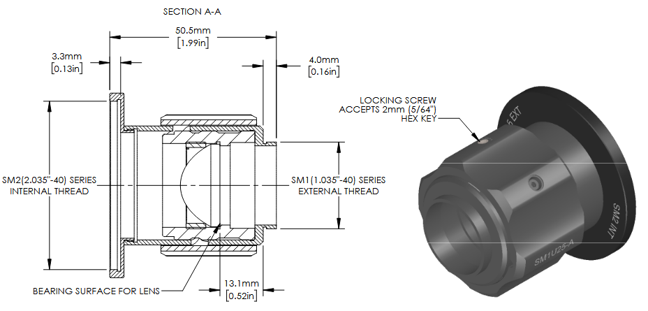
After speaking with a Thorlabs technician, my colleague purchased the following hardware to construct the collimator:
A M450LP2 2W blue LED https://
www .thorlabs .com /item /M450LP2 A SM1U25-A adjustable collimation adapter https://
www .thorlabs .com /item /SM1U25-A
The LED has rectangular dimensions of 1.5 mm x 1.5 mm.
The collimator uses a ACL2520U-A aspheric lens, which has a focal length of 20.1 mm and numerical aperture of 0.6.
I first construct the model of the LED and asphere. I use two object height fields: one on-axis and another at 1.06 mm, which is the half-diagonal of the LED emitter surface.
lens = optic.Optic()

lens.add_surface(index=0, thickness=10.0, material="Air")   # Air gap before lens
lens.add_surface(index=1, thickness=12.0163, material="B270", is_stop=True)  # Planar surface
lens.add_surface(
    index=2,
    thickness=25.0,
    material="Air",
    radius=-10.462,
    conic=-0.6265,
    surface_type="even_asphere",
    coefficients=[0.0, 1.5e-5]  # Aspheric surface
)
lens.add_surface(index=3)

lens.set_aperture("float_by_stop_size", 22.5)

lens.set_field_type(field_type="object_height")
lens.add_field(y=0.0)
lens.add_field(y=-1.06)

lens.add_wavelength(0.45, is_primary=True)
lens.draw(num_rays=3)
plt.show()
WARNING: No extinction coefficient data found for B270.yml. Assuming it is 0.
Collimate the LED
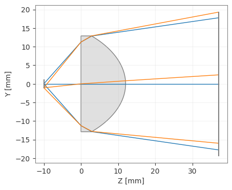
The diverging rays after the lens in the sketch above indicate that the LED is not collimated at this distance from the lens.
To address this (at least initially), I set up an optimization problem to minimize the direction cosines of the rays in the y-direction for the on-axis field. This uses the real_M operand and treats the thickness of the first (object) surface as the variable.
problem = optimization.OptimizationProblem()

# Collimate rays from an on-axis point through different pupil coordinates
for pupil_coordinate in [0.0, 0.7, 1.0]:
    input_data = {
        "optic": lens,
        "surface_number": -1,
        "Hx": 0.0,
        "Hy": 0.0,
        "Px": 0.0,
        "Py": pupil_coordinate,
        "wavelength": 0.45,
    }
    problem.add_operand(operand_type="real_M", target=0.0, weight=1, input_data=input_data)  # Minimize y direction cosines

problem.add_variable(lens, "thickness", surface_number=0, min_val=10.0, max_val=20.0)
problem.info()
╒════╤════════════════════════╤═══════════════════╕
│    │   Merit Function Value │   Improvement (%) │
╞════╪════════════════════════╪═══════════════════╡
│  0 │              0.0345703 │                 0 │
╘════╧════════════════════════╧═══════════════════╛
╒════╤════════════════╤══════════╤══════════════╤══════════════╤══════════╤═════════╤═════════╤════════════════╕
│    │ Operand Type   │   Target │ Min. Bound   │ Max. Bound   │   Weight │   Value │   Delta │   Contrib. [%] │
╞════╪════════════════╪══════════╪══════════════╪══════════════╪══════════╪═════════╪═════════╪════════════════╡
│  0 │ real M         │        0 │              │              │        1 │   0     │   0     │           0    │
│  1 │ real M         │        0 │              │              │        1 │   0.119 │   0.119 │          41.23 │
│  2 │ real M         │        0 │              │              │        1 │   0.143 │   0.143 │          58.77 │
╘════╧════════════════╧══════════╧══════════════╧══════════════╧══════════╧═════════╧═════════╧════════════════╛
╒════╤═════════════════╤═══════════╤═════════╤══════════════╤══════════════╕
│    │ Variable Type   │   Surface │   Value │   Min. Bound │   Max. Bound │
╞════╪═════════════════╪═══════════╪═════════╪══════════════╪══════════════╡
│  0 │ thickness       │         0 │      10 │           10 │           20 │
╘════╧═════════════════╧═══════════╧═════════╧══════════════╧══════════════╛
I use the default optimizer because I don’t see this problem as requiring anything special.
optimizer = optimization.OptimizerGeneric(problem)
optimizer.optimize()
problem.info()
╒════╤════════════════════════╤═══════════════════╕
│ │ Merit Function Value │ Improvement (%) │
╞════╪════════════════════════╪═══════════════════╡
│ 0 │ 2.11412e-05 │ 99.9388 │
╘════╧════════════════════════╧═══════════════════╛
╒════╤════════════════╤══════════╤══════════════╤══════════════╤══════════╤═════════╤═════════╤════════════════╕
│ │ Operand Type │ Target │ Min. Bound │ Max. Bound │ Weight │ Value │ Delta │ Contrib. [%] │
╞════╪════════════════╪══════════╪══════════════╪══════════════╪══════════╪═════════╪═════════╪════════════════╡
│ 0 │ real M │ 0 │ │ │ 1 │ 0 │ 0 │ 0 │
│ 1 │ real M │ 0 │ │ │ 1 │ 0.004 │ 0.004 │ 71.1 │
│ 2 │ real M │ 0 │ │ │ 1 │ -0.002 │ -0.002 │ 28.9 │
╘════╧════════════════╧══════════╧══════════════╧══════════════╧══════════╧═════════╧═════════╧════════════════╛
╒════╤═════════════════╤═══════════╤═════════╤══════════════╤══════════════╕
│ │ Variable Type │ Surface │ Value │ Min. Bound │ Max. Bound │
╞════╪═════════════════╪═══════════╪═════════╪══════════════╪══════════════╡
│ 0 │ thickness │ 0 │ 13.0512 │ 10 │ 20 │
╘════╧═════════════════╧═══════════╧═════════╧══════════════╧══════════════╛
lens.draw(num_rays=3)(<Figure size 1000x400 with 1 Axes>, <Axes: xlabel='Z [mm]', ylabel='Y [mm]'>)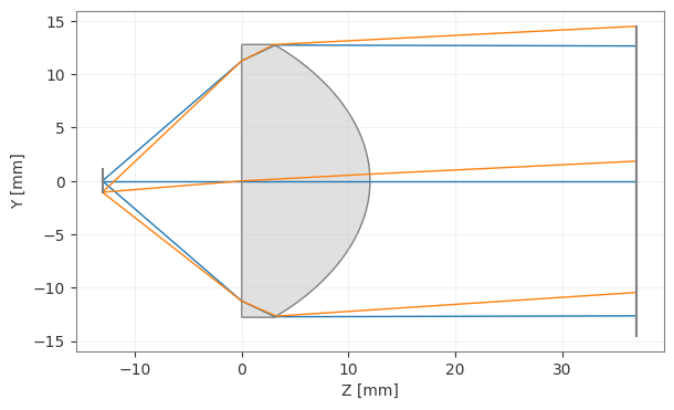
You can see that the lens now lies at a distance of about 13 mm from the LED surface.
As expected, the rays from the on-axis field are now approximately parallel to the axis, and rays from the off-axis field point are approximately parallel as well (though not to the axis, of course).
Interestingly, the schematic provided by Thorlabs for the collimating adapter has a minimum separation distance between the asphere and the LED mounting threads of 13.1 mm. However, this can be extended by up to 11 mm, which suggests that the LED is “collimated” at the position where the lens is closest to the LED and the extension may be used to focus the LED at different distances from the adapter.